AFT Impulse Pulsation Frequency Analysis (PFA) Module

This presentation is prepared by Mr. Deepak Sethia who is working in ImageGrafix Software FZCO, the Hexagon CAS Global Network Partner in the Middle East and Egypt. He has extensive experience in using Caesar II, PV Elite, AFT Impulse software, and troubleshooting. The points that will be covered in this article are:

• Introduction
• Natural Frequency and Resonance
• Piping System Vibration and Resonance
• PD Pump Pulsation
• Overview of PFA for Impulse

Piping System Vibration and Resonance:

Piping systems can vibrate or resonate in two ways

– Through the pipe solid material

• This is called “mechanical vibration”
• If the vibration frequency is at the natural frequency it is called “mechanical resonance”

– Through the fluid inside the pipe

• This is called “acoustic vibration”
• If the vibration frequency is at the natural frequency it is called “acoustic resonance”

PFA PROCESS IN AFT IMPULSE:

PFA Process:

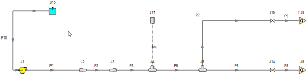
Build the model

– This model represents the suction side of a system with two PD pumps (J8 & J9) in parallel fed by a centrifugal pump (J1)

– We will analyze the upper PD pump (J8)

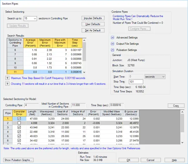
Select Pulsation Setup from the Analysis menu

▪ This is where the “ring” will be defined

– Specify junction (only one in the system) and pulse start time

– The automatic magnitude of the strike will be twice the steady-state flow

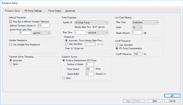
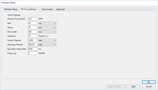
Details of the PD pump are entered on the PD Pump Setup tab

– Used to generate the flow vs. time pump curve for the child pump scenarios

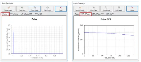
With everything defined we can view the flow pulse that will be used to “ring” the system

– Click Show Pulsation Graphs… in the lower-left corner

The pulse spike and the FFT of the pulse without filtering are shown in the first two tabs

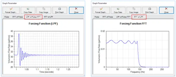
Once the low-pass filter is applied (140 Hz in this case), the pulse spike is now a decaying sine wave

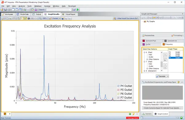
Evaluate Frequencies:

• After running the model, go to the Graph Results window
• Select the new Frequency tab
• Select the pipe location(s) to analyze and click Generate
  • The spikes show the frequencies that excite the system at that location

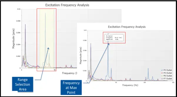
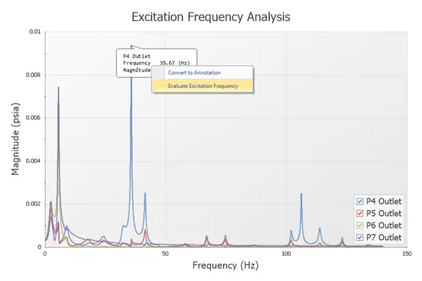
Right-clicking on the annotation brings up a menu, allowing the user to Evaluate Excitation Frequency

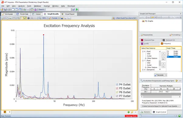
For PD pumps, the speed (RPM) will be determined at that frequency for the harmonic multiples

– A red dot appears indicating the frequency is being evaluated

These scenarios have special properties since they are dependent on the configuration of the parent scenario

• They are read-only so most of the model cannot be changed
  • They will be deleted when the parent is changed
  • They are named with the pump speed and frequency

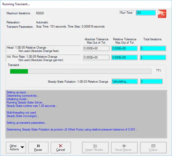
Analysis:

When the model is run, there will be several blocks of time steps used to determine when the model reaches an equilibrium– This eliminates any artificial fluctuations caused by the PD pump flow, and leaves just the steady-state harmonics of the system

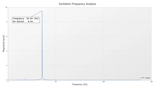
Graphical Report:

The frequency response graph can again be generated– Notice the spike occurs at the frequency of interest.

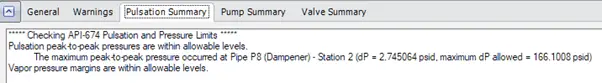
Output Report:

At the end of the run, the maximum peak-to-peak pressure levels are checked against the API-674 standard

– If the levels are OK there will be a confirmation

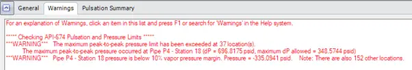
– A warning is given if there are locations that exceed the maximum set by the standard. It will list the location where the largest DP occurred.

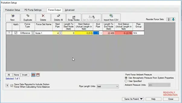
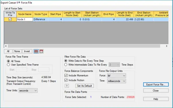
Generate the Force file for CAESAR-II: