What is Process Optimization? | Basics and Techniques of Process Optimization (With PDF)

Process optimization involves the application of mathematical techniques & tools to find out the best possible solution from several available alternatives for the purpose of the maximum Return On Investment (ROI).

The main purposes of process optimization are:

• To increase the productivity with lowest applicable cost.
• To eliminate losses as much as possible.
• To utilize lower cost feedstock, energy with acceptable quality level.
• To maximize the operating capacity of process equipment.
• To design & operate the plant at the most optimum condition. To attain new or most efficient designs and to determine the most desirable operating conditions and safe operation.

So in a sentence, all the above can be mentioned as Process Optimization can increase the production rate to its maximum with maximum profit and minimum waste generation and impact on the environment. By performing process optimization, we aim to obtain the best result under given circumstances.

In this article, we will understand the requirements for process optimization basics and techniques.

Advantages of Process optimization

With process optimization, we get improved plant performance like

• Increase Yield.
• Enhance Availability.
• Reduce energy consumption.
• Reduce maintenance costs.
• Reduce failure in equipment.
• Minimize the unplanned shutdown.

Process Optimization Examples

The following paragraph lists some examples of Process optimization for maximizing profit:

• Design of HEX network (Heat Integration).
• Real-time optimization of a distillation column.
• Model predictive control.
• Operations planning & scheduling.
• Pipeline sizing, Reactor sizing, Distillation column (CAPEX/OPEX).
• Predictive Maintenance (Machine Learning Applications) – Downtime Planning.

The objectives of refinery optimization (TARGET – Maximize Profit) include:

• Minimize crude OPEX at the refinery.
• Optimize refinery crude mix.
• Optimize off-spec generation and optimize overall product mix and dispatch.
• Minimize quality giveaways.
• Optimize fuel consumption, and minimize losses.
• Optimize utilization of the assets.
• Optimize inventory management.
• Optimize capacity utilization and shutdown planning.
• Optimize unit operations maintaining the highest standards of safety, catalyst life, activity, etc.

Process Optimization Framework

• All optimization problems are stated in some standard form.
• One needs to identify the essential elements of a given problem and translate them into a prescribed mathematical form.
• Requirements for application of optimization problem:
  • The design variables.
  • The constraints.
  • The objective (Target) function (Max / Min).
  • The process model.

Process Optimization Framework-Design Variables

The process engineers need to know the design variables that affect the system.

• Example: reactor temp, feed rate, No. of trays In the column, reflux ratio, Batch time, and reactor yield.
• A practical problem may involve many design variables.
• Some of these may be highly sensitive and heavily influence the process being optimized. Choose these as design variables and others (not so-sensitive variables) may be kept constant.
• Note: If all the design variables are fixed, there is no scope for optimization.

Thus one or more variables must be relaxed so that the system becomes an Under Determined System that has at least a principal infinite number of solutions.

Process Optimization Framework – Objective Function

A suitable objective function (cost function) is defined in terms of design variables and often price parameters. The objective function may be technical or economic, which needs to be either maximum or minimum

 Examples of economic objectives:-

• Maximum profit.
• Minimize the cost of production.

 Examples of technical objectives:-

• Maximize reactor yield.
• Minimize the size of the equipment.
• Minimize environmental impact.

Note:- technical objectives (Target) are ultimately related to economics

In a practical process plant, there would be multi-objective functions to be optimized in one case only, therefore, there is more than one objective function.

Process Optimization Framework – Constraints

The constraints request some additional relationships among the design variables and process parameters. The constraints originate because design variables must satisfy certain physical phenomena & certain resource limitations.

Example: Variable bounds: 0<x<1 (Don’t exceed the range in any direction) (Max / Min)

• Equality constraints: The sum of the mole fraction should be unity such as for the component balance equation in a distillation column.
• Inequality constraints: In the packed reactor, the process temp should be less than the catalyst deactivation temp/acidic conditions pH<7, and stress developed anywhere in a component should be less than the maximum allowable stress

Process Optimization Framework – Process Model

• A process model (HYSYS) is required to describe the manner in which the design variables are related. The process model also tells us how the objective function is affected by the design variables.
• A model is a mathematical equation or a collection of several equations that define how the design variables are related and the acceptable values these variables can take.
• Optimization studies are carried out using a simplified (but reasonably accurate) model of a real system.
• Note:- working with a real system (life) is time-consuming, expensive, and risky & that’s why you need to work on a model rather than a life case.

Classification of Process Optimization Methods

Based on the nature of the equation involved, process optimization methods are classified as:-

• Linear Programming (LP)
• Non – Linear Programming (NLP)
• Sequential Quadratic Programming (SQP)

Based on the nature of design variables, process optimization methods are divided as:-

• Continues optimization (Linear Programming)
• Integer programming (IP) (integer values)
• MILP mixed integer (Linear & Integer Programming)
• MINLP (Non-Linear & Integer Programming)

Based on the number of object functions, process optimization methods are grouped as:-

• Single
• Multi

Problem Formulation for Process Optimization

• In order to be able to perform optimization on any process, firstly you will need to formulate the optimization problem.
• In order to formulate a proper optimization problem, you will need to digest the following expressions:
  • Process Models for optimization
  • Degrees of freedom analysis
  • Optimization problems in chemical engineering

Process Models for Optimization

Optimization requires the use of mathematical techniques for maximization or minimization of an objective function (Variable required to be approached – Target).

Note: With the advent of computers, optimization has become part of computer-aided design.

• In order to use optimization algorithms on computers, we must have a quantitative model available to compute the responses of the objective function.

A process model is a set of equations that imitates reality and cannot incorporate all features of the real process. However, a reasonably accurate model saves us time and money as we can avoid repetitive experience & measurements.

Classification of process models:-

• Theoretical Models.
• Database Models (Practical).

Other classifications:-

• Linear vs nonlinear models
• Steady-state vs non-steady state

Degrees of Freedom Analysis for Process Optimization

 The degrees of freedom analysis gives us the number of design variables that can be changed during the optimization process to obtain the optimal solution.

Degrees of freedom, DOF = No. of variables – No. of linearly independent equations (As in Algebra)

• If DOF = 0, a unique solution exists – NO optimization is possible
• If DOF> 0, under the determined system – An infinite solution exist & optimization is possible 
• DOF< 0, over-determined system – No solution exists

Introduction to Linear Programming

Linear Programming is one of the most effective and widely used optimization techniques. A linear programming model seeks to Maximize or Minimize a linear function, subject to a set of linear constraints. The linear model consists of the following:

• A set of design variables
• An objective function is a linear function of design variables
• A set of linear equality or inequality constraints

How do the linear constraints arise?

• Design limitation: For newly established projects the limitation might arise from the design Codes / Standards / Specifications. For existing facilities, the design basis of the facility/asset will identify the limits which have to be respected.
• Production limitation:– equipment limitation, storage limits, market requirements.
• Supply limitation: Raw material / Feedstock limitation
• HSE restriction:– allowable operating ranges for temperature & pressure. Also respecting the environmental legislation with regards to the emissions and effluents generated from the process plant.
• Physical property specification:– product quality constraints when a blended property can be calculated as an average of the pure components.

How to formulate a linear programming model:-

• Determine design variables
• Determine objective function/target
• Determine constraints

Case Study: Hydrocarbon Pipeline Optimization using Simulation

Objective: Optimally determine the best-suited pipeline size considering the material cost of the pipe, pump (CAPEX), and the associated running cost of the pumping system (OPEX).

Constraints:

1. Pipeline ANSI rating 300# and 600#.
2. Pipeline Length 125 km.
3. Diesel design flow of 725 m³/hr.
4. Operational hours of 16 hrs.
5. Potential pipe sizes (X), of 16”, 18”, and 20”.
6. ACCE (Aspen Capital Cost Estimator) for a pipeline cost estimate.
7. APEA (Aspen Process Economic Evaluation) for pump fixed and running cost

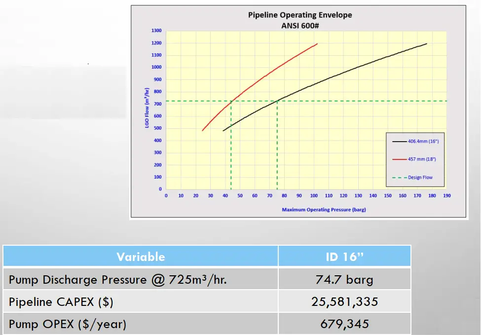
Case 1- Base Case: (Refer to Fig. 1)

• Design Flow 725 m³/hr.
• ANSI rating 600#.
• Operational hours: 16 hrs.
• Pipe ID: 16”.

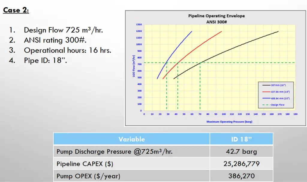
Case 2: Refer to Fig. 2

• Design Flow 725 m³/hr.
• ANSI rating 300#.
• Operational hours: 16 hrs.
• Pipe ID: 18’’.

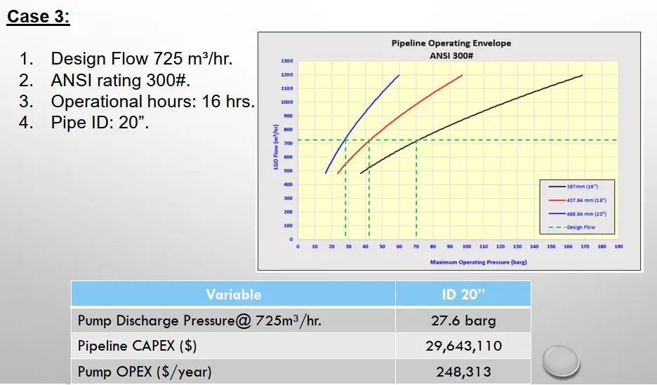
Case 3: Refer to Fig. 3

1. Design Flow 725 m³/hr.
2. ANSI rating 300#.
3. Operational hours: 16 hrs.
4. Pipe ID: 20”.

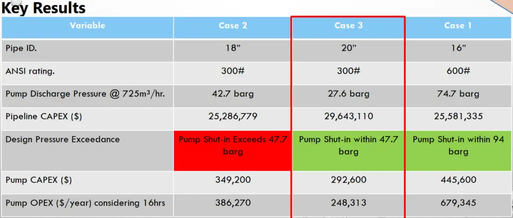
Key Results (Fig. 4):

Conclusions of the above case study

Case 2 can be disqualified where the shut-off pressure of the transfer pump will exceed the design pressure of 47.7 barg.

• Case 1 and Case 3 are technically viable where they meet the Flow requirements and the design pressure of 300# and 600# respectively.
• Case 1 (16” pipeline – ANSI 600#) has reported a lower CAPEX than Case 3 (20” – ANSI 300#), however, the pump cost and electricity cost of Case 1 is higher.
• Although, Case 1 has reported lower pipeline CAPEX, however, it Can be dismissed for the following reasons:
  • Pump opex is nearly three times the value of case 3.
  • Maximum operating pressure under case 1 is 2.8 times of case 3. As a result, the expected peak surge and relieving volume would result in a Bigger SRV size and more relieving volume.

Recommendation

Considering previous technical discussion and outcomes From techno-economic analysis, it is recommended to Case 3 is deemed more favorable and technically viable To cater to the operational requirements (design flow Rate and less surge demand) and more economic Compared to cases 1 and case 2.

Case Study: Tank Area Optimization Using MS. Excel Solver

• Objective

You have to design an open storage tank made of Stainless Steel with a square base. The volume of the tank should be 50 m3.

Find the optimal dimensions of the tank that will require the least material and satisfy the minimum cost.

Problem Formation:

Assume

• X: Length of base
• Y: Height of the tank

The quantity of material will depend on the total surface area of the tank

A = X² + 4XY ————– This is the objective function

Volume is given as a Constraint in the problem statement = 50 m3

Since volume = Area of base * Height

50 = X² * Y

Therefore,

Y=50 / X²——————-equation i

Since the Total Surface Area of the tank  = Area of square + Area of base

Area = 4XY + X², substitute using equation i

Therefore, Area = X² + 4X (50/X²) = X² + 200/X

There are two paths to proceed:

1. Short Path – Semi-Quantitative Optimization.
2. Proper Engineered Path – Quantitative Optimization.

1. Semi-Quantitative Optimization

o Since the equation relating Area to Length is ready, then you can assume various values for X, from 1 to 9, and then plot a curve for X versus Min Area.

o Trend will be as shown below:

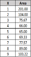
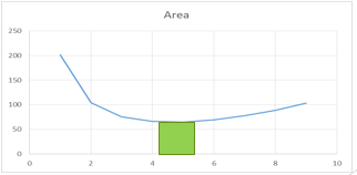
o From the trend you can assume that the minimum area will be associated with a length between 4 – 5 m.

2. Proper Engineered Path – Quantitative Optimization:

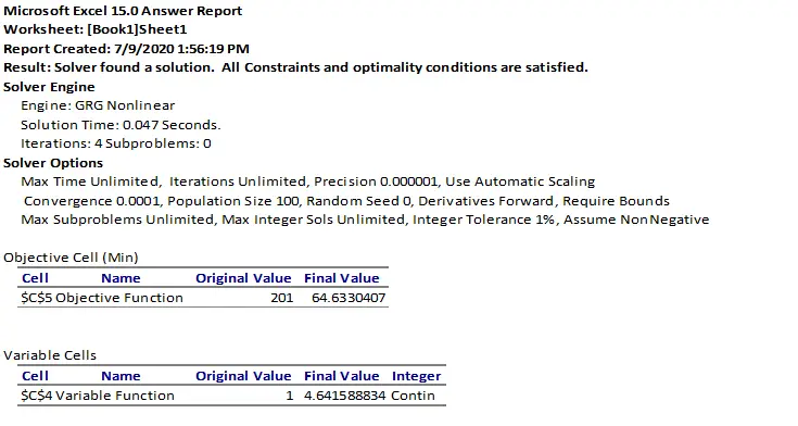
• Use MS Excel Solver to get the accurate values of X & The associated Minimum Area.
• Following the steps of Solver discussed previously, you will get the below results:

Eventually, any engineer should utilize any optimization methodology either to produce an optimized design package or to optimize a running facility.

Always keep in mind that Optimization talks about a few keywords:

1. Maximum Gain.
2. Minimum Loss.
3. Associated CAPEX.
4. Associated OPEX.

Please Note that if there is a shortfall or limitation of this document then it is because of me, while any success or correctness would be solely from the great and generous Allah.