GRE Design Envelope and Failure Envelope

GRE Design Envelope (Failure envelope) is a 2-dimensional (2D) graphical plot of hoop stress and axial stress that provides safe operating conditions of GRE piping/pipeline system when subjected to combined stresses. The hoop stress is plotted in the horizontal axis (X-axis) and the axial stress is plotted in the vertical axis (Y-axis) as shown in Fig. 1. The area surrounded by the lines represents the strength of the GRE piping system. So, if the stress of any component falls within the boundary area, the system will be considered as safe and if the stress falls outside the boundaries, the system will be considered as failed. So, for failed systems pipe stress engineers have to reduce the component stress in some way to bring it within the envelope boundaries. The FRP design envelop is created from the short term and long-term failure envelopes.

For FRP/GRE pipe and pipeline stress analysis the GRP failure envelope curve is significant to extract datapoints for inputs in stress analysis software programs. In this article, we will explain how the GRE design envelope is generated and how to extract data for FRP pipe stress analysis.

**Fig. 1: GRE Failure Envelope and Design Envelope**

Development of GRE/FRP failure envelope starts with the GRE/FPR Qualification process which is covered in ISO 14692 Part 2. In general, several tests are performed, and those material test data are plotted for generating GRP failure envelope.

Development of Short-Term Failure Envelope:

The development of short-term failure envelope needs only two datapoints which are obtained from two different tests as explained below:

Test 1- Short Term Test following ASTM D1599:

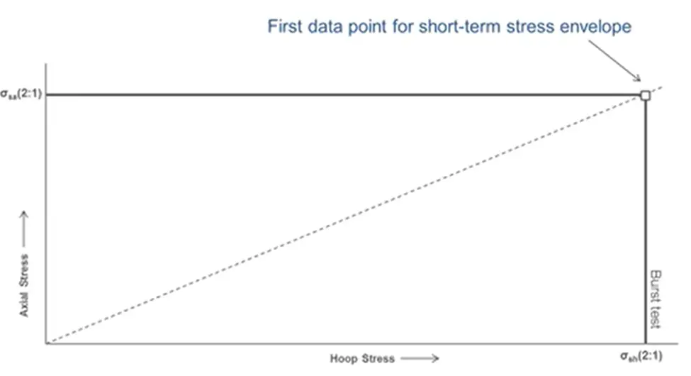
For the short-term test according to ASTM D1599, the pressure inside the test sample is increased until failure. This test is also known as burst test. The pipe test samples are unrestrained, closed ends and the failure usually takes place in 60 to 80 seconds. This generates the first datapoint for short term failure envelope. From the burst test, we get the data for short term hoop stress σ_sh (2:1). Also, as the axial stress is half of hoop stress for pressurized pipes, we get data for σ_sa(2:1). Refer to Fig. 2 below:

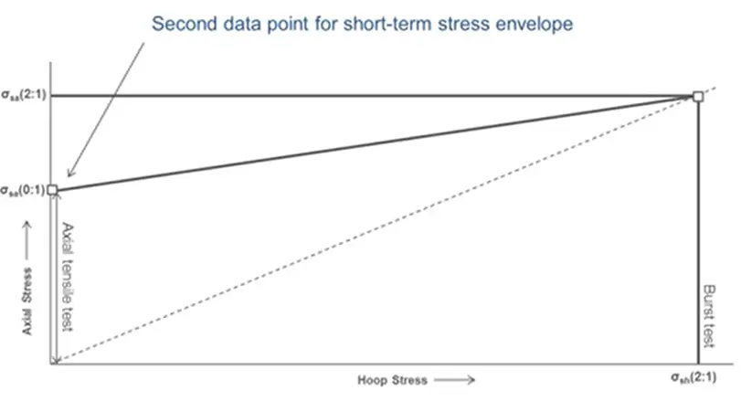
**Fig. 2: First Data Point for Short-Term Failure Envelope**

Test 2-Axial Test (Short-term uniaxial test) following ASTM D2105:

Axial tensile test is to be performed following ASTM D2105 which gives the second data point (Fig. 3) to be included in the FRP design envelope plot. σ_sa (0:1) is the short-term axial stress which is obtained from this test.

**Fig. 3: Second Data Point for Short-term Failure Envelope**

From these two data, we can calculate the bi-axial stress ratio, r which is defined as twice the ratio of σ_sa(0:1) and σ_sh(2:1).

READ How to Avoid Zero Anchor Loads from Piping

r=2* σ_sa(0:1)/σ_sh(2:1)

The bi-axial stress ratio defines the slope of the top line in the GRP pipe failure envelope plot. So, the GRE short-term envelope is created which is defined by two points; short term axial stress σ_sa(0:1) and short term hoop stress σ_sh(2:1). Refer to Fig. 4 below:

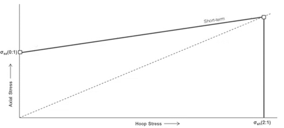
**Fig. 4: FRP Short-Term Failure Envelope**

The short term FRP envelope is generated to deduce the shape of the plot and slope of the top line as the long-term envelope will also follow the same slope.

Development of Long-Term Failure Envelope:

The first datapoint for the long-term GRE failure envelope is obtained from the Regression Test.

Test 3-Regression Test following ASTM D2992:

Full regression test is performed on 18+ GRE pipe samples with different pressures and their time to failure is recorded. The test is performed at 65 Deg C or design temperature when it is higher. The longest test duration is 10000 hours (417 days). The pipe pressure test data is usually plotted in a log stress (vertical axis) – log time (horizontal axis) graph and a line (regression line) is drawn through the cloud of points. Then that line is extrapolated to match 20 years (175400 hours) duration. It will provide the long-term hydrotest pressure (LTHP). The lower confidence limit (LCL) value is obtained by considering a 97.5% confidence limit of LTHP. The LCL signifies the pressure for which we can 97.5% sure that no failure/weepage/leakage will occur at this pressure if we run it for 20 years of lifetime.

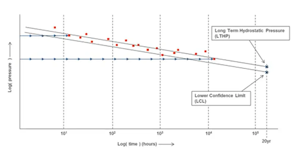
**Fig. 5: Development of LCL/Qualified Pressure from Regression Curve Plot**

On other words, we can say the LCL is the allowable pressure for 20 years design life. It is also known as qualified pressure which can be easily converted to qualified stress using Barlow formula to get qualified stress (σ_qs). This point forms the first data point for the long term failure envelope σ_hl(2:1). The regression test is performed to find out LCL, qualified stress, and baseline gradient.

READ How to Open CAESAR II File in START-PROF?

Test 4:

The second datapoint on the long-term failure envelope is obtained by performing a 1000-hour test with 1:1 load condition. Special arrangements are made to achieve 1:1 load condition. The results are then extrapolated for 20 years following the same regression line achieved during regression test. From this test we will get σ_hl(1:1). This is as per ISO 14692-2017. As per the earlier edition of ISO 14692, the datapoint is derived by finding the exact intersection of 1:1 line with the top line.

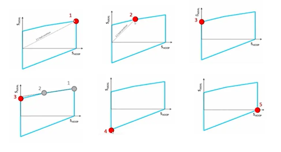
**Fig. 6: Datapoints for long-term failure envelope as per ISO 14692-2017**

The third datapoint for long-term failure envelope (σ_al(0:1)) is obtained by calculating using the following equation; σ_al(0:1)=r* σ_qs/2. In the latest edition of ISO 14692-2017, this data is derived by drawing a straight line connecting datapoint 1 and 2. Then the value obtained due to intersection of the drawn line with the vertical axis is multiplied by 0.8 to get σ_al(0:1).

To get the datapoint 4 for the long-term failure envelope, no material testing is performed. However, the uniaxial compression strength is calculated using the following equation:

σ_al(0:-1)=1.25* σ_al(0:1)

The datapoint 5 is the pure hoop stress under pressurized 2:1 load condition.

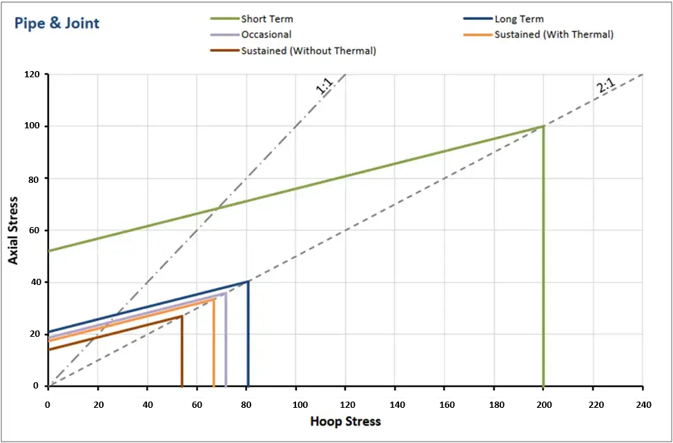
GRE Design Envelop

The GRP design envelop is generated from the long-term failure envelop by reducing the long-term failure envelope by various factors. Initially the factored stress envelope is developed by applying partial factors A1 (temperature), A2 (chemical resistance), and A3 (cyclic condition) as shown below in Fig. 7:

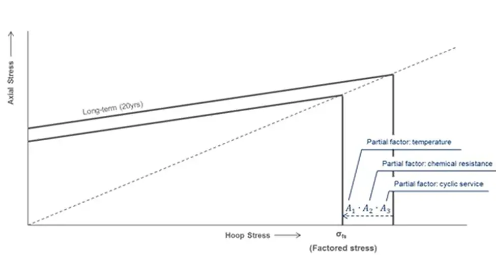
**Fig. 7: Generation of Factored Stress Envelope from long-term failure envelope**

These partial factors are applied because of the differences between test condition and actual operating condition. Next, we apply part factors to get the design envelope from the factored stress envelope to actual FRP design envelope. Depending on loading condition, there are three values of part factors, f₂which signifies a safety factor for different types of loading.

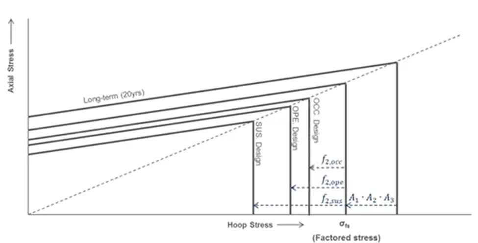
**Fig. 8: Development of Design Envelope from long-term failure envelope**

So, finally we get three design envelopes for three different types of loading conditions; sustained (f2=0.67), sustained with thermal (f2=0.83), and occasional (f2=0.89) loading condition.

READ Details about CAESAR II Error: “Material is Outside the Temperature Range”.

So, the following curve shows all the envelopes in a single plot:

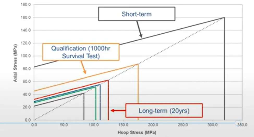
**Fig. 8: GRE Failure Envelope vs Design Envelope**

The 1000 hr. survival test plot (orange color) in this group is only performed for verification purposes.

Typical Example:

Let’s take an example to find out the design envelop values that are required in pipe stress analysis as input. We have the following plot (Fig. 9) from the manufacturer.

**Fig. 9: Typical FRP Failure Envelope from Manufacturer**

For Caesar ii GRE pipe stress analysis, we need to enter the following data which has to be extracted from the long-term failure envelope plot.

**Fig. 10: Data Required in Pipe Stress Analysis software Caesar II**

You can easily measure the data from the above long-term failure envelope plot. In general, for accuracy purposes vendor provides these data in a tabular format.