What is Time History Analysis? Steps with example

Time history analysis is quite popular in pipe stress analysis as it provides the most realistic specification of dynamic loads in CAESAR II. The program’s modal time history analysis can simulate system response to several force-versus-time events. Time history is best suited to impulse loadings (slug, water hammer, PSV reaction, etc.) or other transient loadings where the profile is known.  Only one dynamic load can be defined as a time history analysis. This dynamic load case can be used in as many static/dynamic combination load cases as necessary. The single load case may consist of multiple force profiles that can be applied to the system simultaneously or sequentially. Each force versus time profile is entered as a spectrum with an ordinate of Force (in current units) and a range of Time (in milliseconds). The profiles are defined by entering the time and force coordinates of the corner points defining the profile. In this article, we will explore the methods followed for dynamic time history analysis using Caesar II considering an example of a slug flow system.

Reason for Dynamic Time History Analysis

While the adoption of a pseudo-static approach, the application of a static load corrected using an appropriate dynamic load factor, can also provide a conservative result. In some short pipe routing it is required to check how the pipe routing responds to loads with very short durations. This is why time history analysis is often considered a better approach and can be performed with commercial software such as CAESAR II.

Time history analysis provides a method of assessing displacements, stress, and reactions developed in a piping system over time. In order to carry out such an analysis there is a need to be able to define the loading, be it the forces associated with a fluid slug traveling through a piping system.

Time History Analysis Example using Caesar II

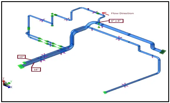
In the following paragraphs, we will discuss the time history analysis for the design of a Flowline of a typical Wellhead piping system. The pipeline system shown in Fig. 1 is used for dynamic time history analysis.

Time History Analysis Input

Time history analysis input can be divided into three steps listed below:

1. Modification in the Static Model
2. Dynamic Load Definition and
3. The setting of Dynamic Control Parameters

1. Modification in the Static Model

Element length needs to be kept at a minimum for getting proper mass distribution, mode shapes, and natural frequency of the system. The following thumb rule for maximum element length can be followed:

• Minimum of 10 times of nominal diameter i.e 10D and 6000 mm.
• 5 times of nominal diameter near anchor or line stop supports.
• at least 1 node in between two supports.
• At least 1 node between two bends.

Support stiffness values can be considered to get more accurate results.

2. Defining Dynamic Loads for Time history analysis

The main inputs required to enter the spreadsheet for dynamic time-history analysis are listed below:

• Slug Force can be calculated by collecting fluid density and velocity from the Process department.
• The time duration for traveling from one elbow to another can be calculated by dividing the pipe length between two elbows by flow velocity. Two-time durations need to be calculated. Those are slug duration and slug periodicity. Both of these time durations will be required to create a time history spectrum for analysis. So, before opening the caesar ii dynamic input module, Calculate slug force, slug duration, and periodicity for each elbow node where the slug is expected to hit.

Let’s move on to the actual caesar ii time history analysis module. Before starting the dynamic module the static analysis need to be performed and the system must be safe in all static stress analysis aspects.

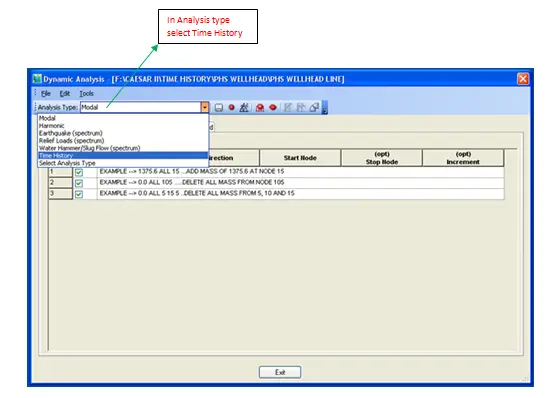
Step 1-Starting the Time history module: Open the Caesar II time history module as shown in Fig. 2

Step 2- Force Time profile definition: Refer to Fig. 3 below to understand the node numbers of the system.

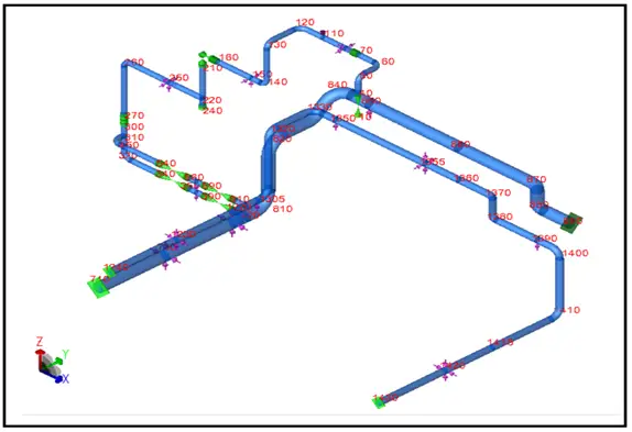
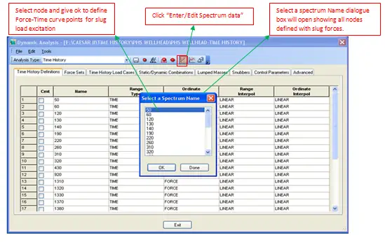
Slug force needs to be applied in each elbow node (50, 60, 120, 130, 140, etc) as shown in the above system. For each elbow node, force-time profile is to be created for time history analysis. As shown in Fig. 4 enter values corresponding to each elbow node.

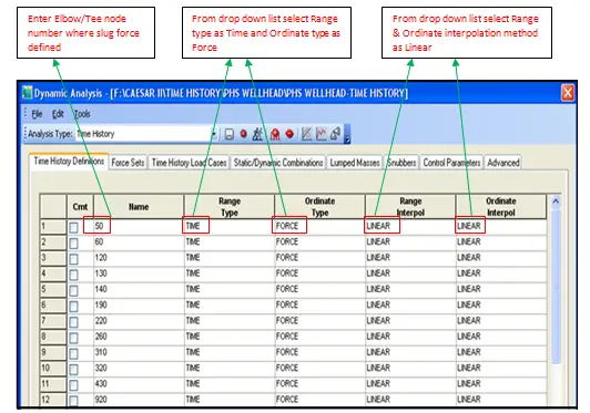
Input Range type as time, Ordinate Type as Force, Range Interpol, and Ordinate Interpol as Linear. Now click on the highlighted button (Fig. 5) for generating a time-history profile for each node entered in Fig. 4.

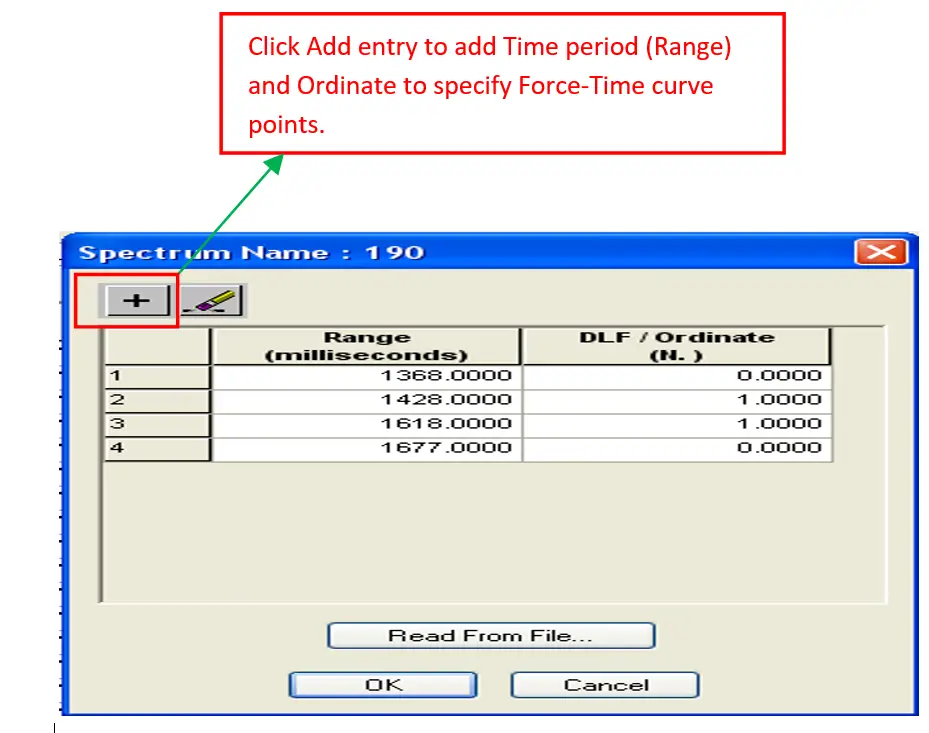
Now select each node one by one and enter the earlier calculated time and force values to generate a spectrum for each node as shown in Fig. 6 below:

Further steps of creating Force Sets, Time history load cases, and static-dynamic load combinations are the same as explained in the earlier article “Slug Flow Analysis Using Dynamic Spectrum Method in Caesar II“. Kindly click on the link provided to learn the same.

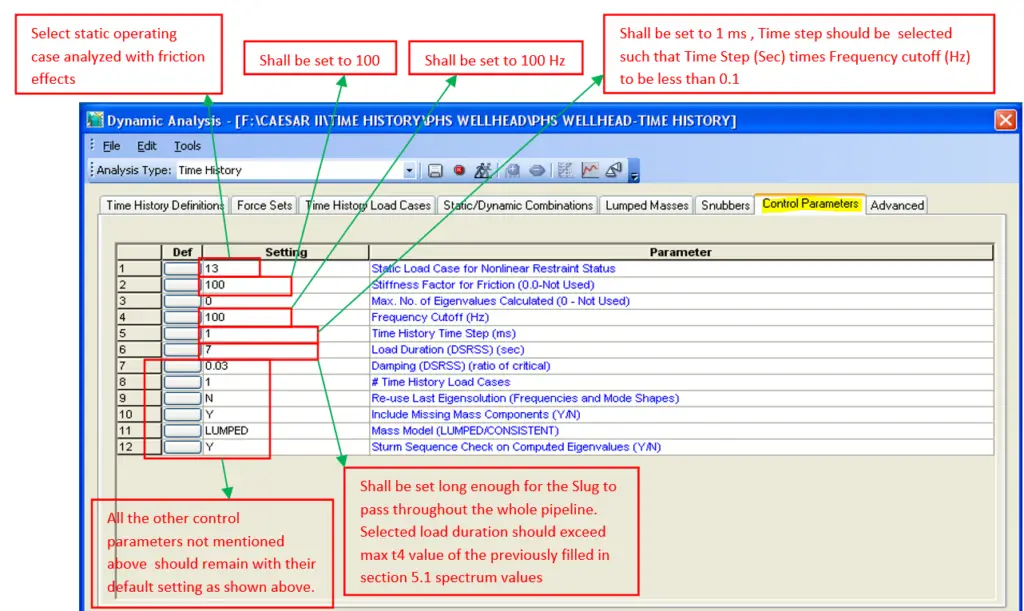
3. Setting up the Dynamic Control Parameters

The control parameters can be set as provided in Fig. 7

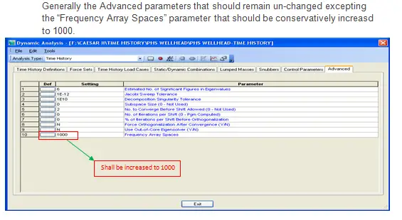
The Advanced control parameters can be set as provided in Fig. 8

Once the input parameters are entered and the control parameter is set up as explained above, run the analysis to get output results. The output results to be checked are similar to the earlier article titled “Slug Flow Analysis Using Dynamic Spectrum Method in Caesar II“

Response Spectrum vs Time History Analysis

The response spectrum method is a linear dynamic analysis method but Time history analysis is normally a non-linear analysis. Time history is a more detailed analysis involving the time instant.

In time history analyses the structural response is computed at a number of subsequent time instants. In other words, time histories of the structural response to a given input are obtained as a result. In response spectrum analyses the time evolution of response cannot be computed. Only the maximum response is estimated. No information is available also about the time when the maximum response occurs.