Dynamic Analysis of Piping Systems

Dynamic analysis refers to the evaluation of how a piping system responds to dynamic loads. These loads can cause vibrations, stress fluctuations, or transient forces that static analysis cannot adequately capture. The main purpose of dynamic analysis is to ensure the safety, reliability, and integrity of piping systems under dynamic conditions and to prevent failures due to fatigue, resonance, or transient overloading. Some of the typical dynamic loads are seismic activity or earthquakes, water hammer or pressure surges due to sudden valve closures or pump trips, slug flow, pulsation from compressors or reciprocating machinery, wind or wave loads, vibration from rotating equipment, etc.

What is Dynamic Analysis of Piping System?

Dynamic Analysis is the study of a fluid-filled piping system to find the system response with respect to time. The dynamic behavior of the piping system is completely different from the static behavior. In static analysis, as the piping system gets enough time to respond against the unbalanced force, the static analysis does not create much problem. But in dynamic analysis, the impact of forces is quick, and the unbalanced force can create havoc causing the piping system to fail. In this article, we will explore the basics of dynamic analysis.

Static Analysis vs Dynamic Analysis

As stated earlier, the system response is completely different in both static and dynamic analysis. The main differences between the two analysis methods are tabulated below:

Static Analysis	Dynamic Analysis
Static Analysis is not dependent on time	The dynamic analysis depends on the time
In static analysis, the acceleration is negligible	Effects of acceleration are considered in dynamic analysis.
In static analysis, the piping System is in equilibrium with balanced forces	The piping System is not in equilibrium in dynamic analysis, and it has unbalanced forces.
Boundary conditions are not dependent on time in static analysis.	Boundary conditions are time-bound in dynamic analysis.

In simple terms, a static load can be considered as a dynamic load with a long duration so the piping system can fully respond to it. In static analysis, force is not dependent on time and acceleration is negligible. Also, the time when it started is not important. The piping system is in equilibrium having balanced forces in the system and the boundary conditions are not dependent on time. It is believed that the load is applied very slowly and that the effect of time is negligible and not considered.

Whereas, in dynamic analysis, the load depends on time. The effect of acceleration is considered in dynamic analysis. Dynamic loading tends to increase the response of the structure beyond the response obtained if the same load is applied statically. The piping system is not in equilibrium, and there are some unbalanced forces between the pipe and the supports supporting it. The response of the system depends not only on the magnitude of the applied force but also on the frequency (i.e., the timing of the load).

Dynamic Modal Analysis

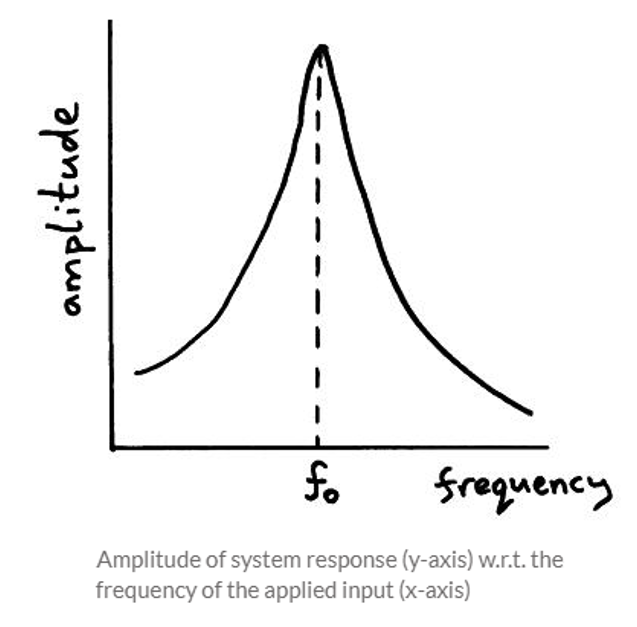
Every system has resonant frequencies, or the ability to vibrate at certain frequencies, without any external load being applied. The amplitude of the response is measured with frequency and as we approach the resonant frequency, the response becomes infinite, as can be seen from Fig. 1. With modal analysis, we are interested in the limits of the response of the system being analyzed. The natural frequencies are found using a stiffness matrix, Eigenvectors, and Eigenvalues. It is important for the users to understand why these frequencies are important and how to set up and analyze modal analysis in to get correct dynamic results, considering all possible parameters. When the natural frequency of the system coincides with the frequency of the externally applied load (that may be any dynamic load like wind, earthquake, slug force, pump vibrations, etc.) resonance condition occurs that leads to substantial damage to the system.

Examples of Resonance causing damage

Here are some examples of resonance creating direct damage to the system.

1985 earthquake in Mexico City

The energy released during this earthquake was equivalent to 1114 nuclear detonations, and the earthquake was felt as far as Los Angeles. Up to the 1950s, no earthquake codes existed. It wasn’t until the later 1950s and 1970s that earthquake codes were developed and introduced for building construction. Despite this, none of these safety precautions accounted for an earthquake.

During the earthquake, most of the 6 to 15-story high-rises collapsed (Fig. 2), resulting in a huge loss of life and property. Interestingly, buildings with less than 6 or more than 15 stories were not damaged as much, while buildings with 9 stories were destroyed to rubble! Two explanations were offered for the earthquake’s impact: the long duration of the shaking and the resulting resonance with the lakebed sediments. In other words, the resonant frequency of the 6 to 15-story structures coincided almost exactly with the frequency of the earthquake.

Tacoma Narrows Bridge – 1940 Disaster

Another real-life example is the Tacoma Narrows Bridge in Washington.

In November of 1940, the bridge instantaneously collapsed.  Investigation of the disaster revealed that the cause of the collapse was an aeroelastic flutter, or it was a wind-induced collapse.  The winds were blowing at a particular frequency, which happened to coincide with the resonant frequency of the structure, resulting in the sudden collapse of the structure.

Example of Resonance in Daily Life

We observe resonance examples in our day-to-day life as well.

The most familiar example is the playground swing. When we push the swing, it starts moving forward and backward. If a series of regular pushes are given to the swing, its motion can be built. The person who is pushing the string has to match the timing of the swing. The pusher has to sync with the timing of the swing. This causes the motion of the swing to have increased amplitude so as to reach higher. Once when the swing reaches its natural frequency of oscillation, a gentle push to the swing helps to maintain its amplitude due to resonance. We call this in-sync motion “Resonance.” But, if the push given is irregular, the swing will hardly vibrate, and this out-of-sync motion will never lead to resonance, and the swing will not go higher.

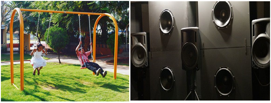
You may also have noticed that the walls and furniture of your home vibrate when you play music on a heavy beat. This is because the natural frequency of the furniture gets resonated with the frequency of the sound of the music, and, hence, causes them to vibrate.

Dynamic Equation of Motion

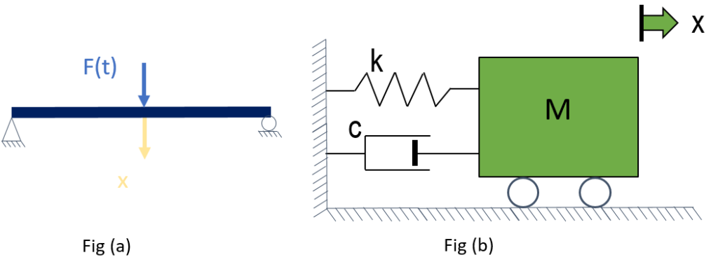
Figure (a) shows an example of a structure represented for dynamic analysis as a single-degree-of-freedom system i.e. structure modeled as a system with a single displacement coordinate. This single degree of freedom system is described conveniently with the mathematical model as shown in Figure (b) and can be written in the equation also called as ‘Dynamic Equation of Motion‘

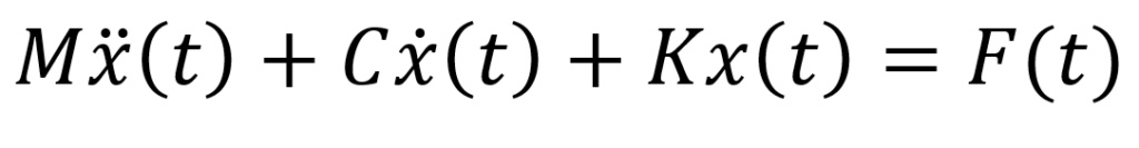
Fig (b) has the following components

1. Mass element m represents the mass and inertial characteristics of the structure
2. Spring element k represents the elastic restoring force and potential energy capacity of the structure
3. A damping element c represents the frictional characteristics and energy losses in the structure
4. And an excitation force F(t), representing the external force acting on the structural system

In the adoption of a mathematical model, it is assumed that each element in the system represents a single property, i.e., mass m represents the property of inertia, spring stiffness k exclusively represents the elasticity, whereas damper c represents energy dissipation. Such pure elements do not exist in the physical world, and this mathematical model is a conceptual idealization of the real structure

As the effect of frictional forces or damping is small, we are going to neglect it to explicitly solve this dynamic equation of motion. In addition to this, we consider the system, during its motion or vibration to be free from external action or forces or simply we can say under free vibrations.

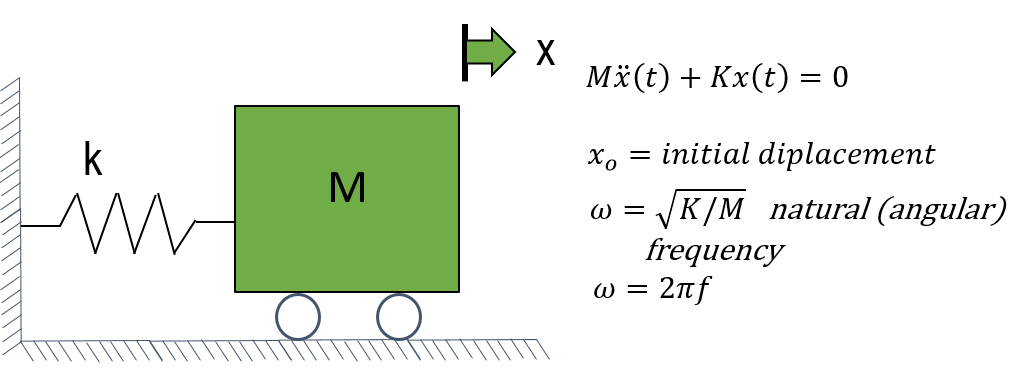
Under this condition, the system in motion is governed only by the influence of the initial condition i.e., displacement and velocity at time= 0. It is represented as xo here. By further solving this second degree of differential equation, we can find a solution for the angular frequency.

Once we get this angular frequency, the cyclic frequency can be calculated as 2 pi f. We can observe that the system characteristics of an SDOF oscillator can be completely described by its Natural Frequency and its damping value.

The free vibration response of any system with N degrees of freedom is the sum of N independent cyclic functions, known as modes of vibration, and each one has its own Natural Frequency and a single degree of freedom. The advantage of this is that each mode is independent and responds to external loads in the same way that an SDOF oscillator does.

Lumped mass model

In pipe stress analysis software, dynamic analysis is performed according to the finite element analysis (stiffness) method using a lumped mass model. With a lumped mass model, the mass of a particular pipe length is lumped at the endpoint only and not distributed equally along the pipe length. The flexible point needs a lower frequency, whereas a rigid point needs a higher frequency to extract your response. Hence, there are chances of missing responses at these rigid points. In real-life complex stress models, this becomes a severe problem due to the number of rigid supports and rigid points in the model.

In order to capture the spatial distribution of the inertial loads, the system must be properly discretized. This can be achieved by ensuring that mass points in the system are properly spaced. If this criterion is not satisfied, additional mass points should be added to refine the model. The time required to insert these piping points can be time-consuming and hence not reasonable for complex models.

Automatic Model Discretization in AutoPIPE

AutoPIPE provides options for refining a model automatically without having to define additional points. The system model is refined by generating mass points during the solution. These points are treated just like other points during the solution; however, they are not accessible for any other purpose. These points will not serve any function other than to provide better mass distribution of the model for dynamic loads.

If the initial distance between two adjacent points is greater than the optimum element length (Lopt), mass points are inserted in order to make the actual distance between points less than or equal to the optimum spacing.

The optimal length is calculated using Roark’s equation for a simply supported beam at both ends and dividing this value by 2 to refine it even further (refer to AutoPIPE help for detailed procedure).

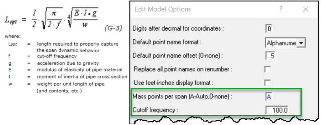
In AutoPIPE, the setting is available (Fig. 5) for this under the Edit model option as ‘Mass points per span’.

If 0 is entered, no mass point discretization will occur. This is the default.

If a value greater than 0 is entered, AutoPIPE will generate that number of mass points spaced equally between piping points (valid range is 1-9).

If A is entered, the number of mass points spaced equally between any two piping points will be generated automatically based on the dynamic properties of each pipe span and on the value entered in the “Cutoff frequency” field.

This cutoff frequency input is only available for input if Auto is entered for the “Mass points per span” field. The value entered at this prompt is used to determine the maximum number of mass points to be generated by AutoPIPE along a span of pipe and should (approximately) match the frequency of the biggest mode shape captured in the modal analysis.

We always recommend selecting ‘Auto’ to get more accurate results.

Modal Analysis in AutoPIPE

1. Open Model in AutoPIPE from, File>Open.
2. Go to Tools > Edit Option and make these changes:
   • Mass point per span (A-Auto, 0-None): A
   • Cutoff frequency: 100 (Fig. 7)

Then click OK to accept.

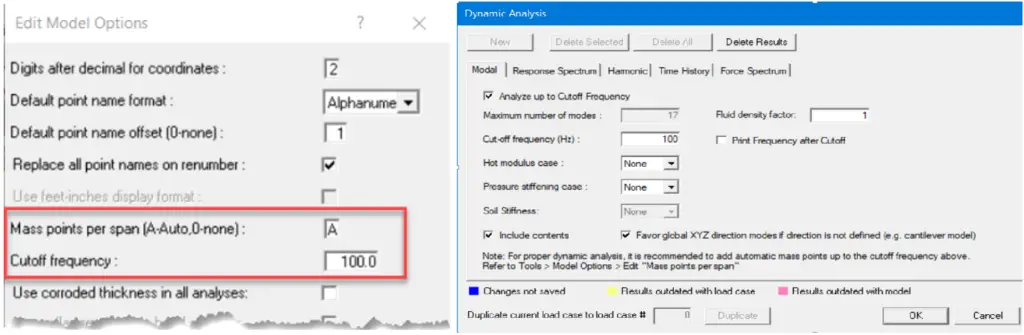
Note: Specifying ‘A’ means that the mass spacing will be applied automatically using a frequency of 100Hz. It is possible to split each length into the same number of spans by using a number in the range 1-9 instead of A, but this can lead to very closely spaced nodes in short lengths.

3. Go to Analysis > Dynamic analysis (Fig. 7) to set up dynamic analysis settings. Under Modal analysis, check on Analyze up to Cutoff frequency and Provide cutoff frequency value. Review other information if you want to make modifications over there. And then click ‘OK’
4. Then click on Analyze all from the Analysis ribbon. Make sure that Modal analysis is selected and click ‘OK’
5. To graphically review modal analysis results, go to Result > Interactive > Mode shapes. You can also animate these mode shapes to check the orientation of modes.
6. You can also get detailed reports in text format. Go to Result > Output Report, select Frequency & Mode Shapes report, and click ‘OK’.

Results and Interpretation

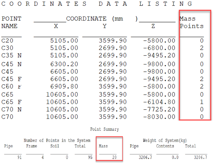
AutoPIPE has automatically inserted intermediate-mass points as per minimum optimal length calculated from Roark’s formula as selected Auto for mass points per span in Edit Model Option.

You can also review the number of mass points inserted under each component by AutoPIPE from the Coordinate data listing. And can also review the total number of mass points (Fig. 8) from the Point summary report.

AutoPIPE reports the same natural frequency for a particular piping system irrespective of the number of nodes in the system. Though you have a break element in-between, there won’t be a considerable change in natural frequencies. That issue you may have faced with our competitor software.

Output reports show these two reports for modal analysis. The frequency section lists the currently active range of natural frequencies calculated for the system by modal analysis. And Mode Shapes section lists the translation (mass normalized), and rotation point displacements for each active mode shape. These are not actual displacements, but the relative response if the system is excited from an external source.

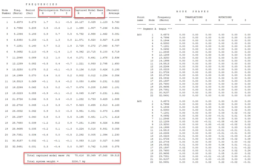
In the frequency report, you will see columns for participation factors and captured modal mass. 

The participation factor is a measure of the importance of the mode. The method used for calculating the participation factors is outlined in the program help. The mass participation report illustrates how sensitive each of the piping system’s modes is too dynamic loading. High modal participation factors indicate that the mode is easily excited by the applied dynamic forces. If subsequent displacement reports indicate high dynamic responses, then the modes having high participation factors must be dampened or eliminated. Once a particular mode is targeted as being a problem, it may be viewed in the mode shape report, or graphically via the animated mode shape plots.

The captured modal mass is another way of quantifying the importance of the mode and the two are related. The captured modal mass percentage tells how much of the response is attributed to a particular mode and also tells the mode orientation (X, Y, or Z). The more of the total system mass that is accounted for, the better is results. Due to the complexity of some piping systems, there may be a large number of DOFs and therefore insignificant modes, that would require a long solution time and it isn’t always practical to do this. We would want to achieve at least 75-80% where possible. But we need to use our engineering judgment on what percentage of captured mass is required and to decide how high to run on frequency.

Static Correction Methods

In order to capture the total dynamic response of a system, all modes of vibration in a system must be considered. The number of modes in a system is equal to the number of mass degrees of freedom in the system, so a typical system will have hundreds of modes of vibration. Modes whose frequency is close to the excitation frequency contribute the most to the response. For many dynamic loadings, the response of the system can be accurately predicted by considering the response of the first few modes. However, higher frequency modes may have a significant contribution to the response at a higher frequency.

Earthquake loading is a relatively low-frequency phenomenon and thus it is usual to only consider modes up to 33 Hertz. Higher frequency modes will not be excited significantly. Harmonic and impulsive loadings, on the other hand, may have high excitation frequencies and hence may excite higher frequency modes. For such loading, all modes with frequencies at least up to the excitation frequency should be extracted.

The extraction of all modes in a large system model can be logistically impractical. However, if only the first few modes of vibration are considered, the remaining modes which are neglected may cause a truncation error. This error is most noticeable in element forces and support reactions. The response of these modes can be approximated by applying a static correction. The amount of correction depends on the system and the excitation. All modes that are important to the response of a certain loading, should be extracted.

Static correction methods are approximate methods and may not be able to predict local responses. AutoPIPE provides the ability to perform two static correction procedures (Missing Mass, and Zero Period Acceleration).

By including Missing Mass Correction in the analysis, the following procedure is followed:

• The amount of mass captured by all extracted modes is subtracted from the total mass.
• The uncaptured mass is subjected to an acceleration equal to that at the cut-off frequency.
• This uncaptured mass is considered another mode and combined with the others using the specified combination method selected.

The inclusion of Zero Period Acceleration (ZPA) can correct these missing modes and follows this procedure:

• The entire structure mass is subjected to the peak ground acceleration
• The static response is obtained for the structure
• The larger the static and dynamic response is reported

In general, the missing mass method is more accurate than the ZPA method. The ZPA method is generally more conservative. Using either method is preferable to a truncated modal solution with no correction. Using both methods together is not recommended as it produces overly conservative results.

Few more related article for you:

What is Modal Analysis: Modal Analysis Example
What is Acoustic-Induced Vibration or AIV?
Flow-Induced Vibration (FIV)
Basics of Vibration Monitoring: A presentation
Piping Vibration: Causes and Effects
Solving vibration problems in a two-phase flowline

Recorded Webinar on Dynamic Analysis

The above article is prepared by Mr. Manoj Kale, Application Engineer in Bentley Systems. He presented the above subject in a webinar. Register here to watch the webinar and learn directly from the expert.

Online Course on Fundamentals of Dynamic Analysis (Caesar II)

There is a very good online course available on Fundamentals of Dynamic Analysis that explains the background theories and application of dynamic analysis using the Caesar II software. It covers the following details:

• Single degree of freedom –Undamped system
• Critically damped system
• Overdamped system
• Underdamped system
• Forced vibration
• Solution to the equation for forced vibration
• Responses in forced vibration- with and w/o damping
• The relation between phase and resonance
• Multi-degree of freedom MDOF
• Expanded version of the MDOF Matrix equations.
• Example to demonstrate the concept of mass and stiffness matrices
• Damping models
• Harmonic analysis- Caesar II
• Response spectrum
• Dirac delta function and impulse response function
• Response to arbitrary force
• Response to step force
• Response to half-cycle sinusoidal force
• Response to symmetrical triangular pulse
• Eigenvalue problem and Concept of modal orthogonality
• Physical meaning of the matrix of mode shapes
• Dynamic analysis of seismic inertial loading-Time history
• Concept of ground motion and structural response
• Mass participation percentages
• Seismic response spectrum analysis
• Seismic displacement spectrum and pseudo-acceleration spectrum
• Concepts in seismic response spectrum analysis
• Analysis of Seismic loads –Calculation of seismic inertial loading from ASCE-7-2022
• Concept of ductility reduction factor
• Seismic analysis- Inertial load calculation
• Response spectrum, modal, spatial, and directional combinations
• Seismic response spectrum in CAESAR II
• Load cases – seismic spectrum
• Control parameters and advanced control parameters
• Highlights from the upcoming B31E on modal and directional combination methods
• What is Seismic anchor movement?
• Seismic analysis results- participation factors
• Shock or Dynamic load factor spectrum for multi-degree of freedom systems
• Force spectrum method
• Fluid hammer –pressure variation
• Force vs time- data used to generate DLF spectrum
• Time history analysis- Caesar II Input and Output
• Wilson theta method
• Fourier transformation
• Random Vibrations
• Probability distribution function
• Concept of expectation values, variance, std. deviation and autocorrelation function
• Concepts and equations relevant to frequency domain analysis
• Broadband and white noise
• Concept of impulse response function
• Concept of input-output in frequency domain analysis
• Measurement of vibration
• Key objectives of the measurement of vibration
• A schematic of vibration measurement of a rotating machine
• Key points for consideration when measuring vibration
• Displacement transducers
• Velocity transducers
• Seismometer and its working principle
• Principle of the accelerometer
• The overall scheme for signal processing
• Schematic for data collection and analysis
• Analog to Digital conversion
• Nyquist frequency
• Aliasing
• Filtering- Low-pass, High-pass, and Band-pass filtering
• Windowing
• RMS VALUE
• Crest factor and Kurtosis
• Discrete and Fast Fourier Transform
• Importance of segment size in FFT
• The concept of averaging
• Power spectral density
• Averaging of spectra
• Concept of overlapping
• Short-term Fourier transform(STFT)
• Proximity probe and orbit plot
• Bode plot and Polar plot
• 2D & 3D Waterfall spectra
• Vibration measurement in bearings and shaft-rotating equipment
• Causes of vibration in rotating machines
• Misalignment types
• Piping vibration- Energy Institute Guideline
• Dynamic strain measurement
• Viscous dampers
• AIV-Theory
• FIV-Theory
• Concepts and examples of fluid dynamics, monopole, dipole, and quadrupole
• Beam and shell modes of vibration

If you are intersted for that course, you can enroll by visiting the following webpage: https://www.everyeng.com/learn/12af6c82/

Questions and Answers from the Fundamentals of Dynamic Analysis Course

Q1. Explain the term degree of freedom with an example. Why is the word ” independent” used in the definition? 

Ans: The degree of freedom means the number of independent ways by which a point can be displaced. The word intendent means, for e.g. Displacement in x direction is say not dependent on displacement in y direction. In terms of CAESAR II, when we say each node has 6 degrees of freedom, all we mean is that the node can have dx, dy,dz,rx,ry,rz movements and these are not dependent on each other.

Q2. Explain the terms mass matrix and stiffness matrix?

Ans: Imagine a structure of N DOFs. If we give unit acceleration to a DOF then the inertia forces that develops in all the DOFs forms a column of a mass matrix. If the process is repeated for all DOFs, then we get the complete mass matrix. Similarly, if we apply unit displacement by that we mean translation or rotation to a DOF and keep all other DOFs fixed then the forces /moments that develop in all DOFs forms a column of the stiffness matrix. Repeating this process for all DOFs generates the stiffness matrix.

Q3. What is meant by mode shape? 

Ans: The pattern of deformation of a body when its vibrating in a particular natural frequency.

Q4. What is modal orthogonality and what is its use? 

Ans: Modal orthogonality mathematically means that the matrix multiplication

Physical meaning- inertia forces for n th mode does zero work in going through r th mode displacements. Stiffness force for n th mode does zero work in going through r th mode displacements.

Q5. Explain how phase angle Changes with damping ratio?

Ans: Its 90 degree at w/wn i.e. at resonance and changes 180 across the resonance situation.

Q6. Explain key differences between overdamped, underdamped and critically damped system?

Ans: Overdamped is when ratio of damping to critical damping is >1. When this ratio is 1.0, its critical damping. When this ratio is less than 1.0 its underdamping. Both overdamped and critically damped system shows exponential decay of amplitude of vibration. Underdamped systems show sinusoidal behaviour with reducing amplitude with every cycle.

Q7. How does damping affect response? 

Ans: By reducing amplitude of vibration and introduce phase difference between input and response.

Q8. What is the key difference between lumped and consistent mass matrices?

Ans: Lumped mass matrices are diagonal. Consistent mass matrices are not diagonal. Consistent mass matrices are based on the satisfaction of physical laws of nature; lumped mass matrices are based on approximately sharing mass into equal proportions between DOFs.