Engineering codes and standards evolve continuously to reflect advances in engineering practice, improved safety philosophy, and lessons learned from operational experience. The 2024–2025 code revisions across major pressure equipment and welding standards represent one of the more significant updates in recent years for the pressure vessel, piping, and welding community.
Recent updates to ASME Boiler and Pressure Vessel Code Section VIII, ASME B31.3 Process Piping Code, ASME B31.1 Power Piping Code, ASME Section IX Welding and Brazing Qualifications, and AWS D1.1 Structural Welding Code – Steel were highlighted during the 2024–2025 Code Changes Webinar hosted by CEI, Paulin Research Group, and Finglow. The webinar link is provided towards the end of the article.
These updates affect pressure vessel design, piping design and stress analysis, welding qualifications, fabrication procedures, and inspection practices. For engineers and designers working in oil & gas, petrochemical, power generation, and heavy fabrication industries, understanding these changes is essential to ensure compliance and maintain design reliability.
Updates in ASME Section VIII (2025): Pressure Vessel Code
1. Responsibility Changes – Appendix 47
- One of the most notable changes involves Appendix 47, where the phrase “responsible charge” has been removed.
- Previously, the code required that vessel design be performed under the “responsible charge” of a qualified engineer. The updated revision shifts the responsibility framework:
- Design personnel must now meet minimum qualification requirements defined within the manufacturer’s quality control system.
- The code itself is less prescriptive about designer qualifications.
- Responsibility shifts more directly to the manufacturer and their quality management program.
- This reflects a broader industry trend toward organizational accountability rather than individual certification language within codes.
2. Increasing Alignment Between Division 1 and Division 2
- Historically, Division 1 provided simpler design rules, while Division 2 offered more rigorous and analytical methods.
- Recent revisions continue a “common rules” alignment effort, which includes:
- Directing more design methodologies toward Division 2 calculation procedures
- Expanding cross-references between the divisions
- Encouraging engineers to apply advanced stress-based design methods
- Design areas moving toward Division 2 methodologies include:
- Flange design
- Expansion bellows
- Jacketed vessels
- Reinforcement calculations
- For engineers accustomed to Division 1 approaches, familiarity with Division 2 methods is becoming increasingly necessary.
3. Paragraph Rewrites and Structural Changes
The 2025 revision includes significant editorial restructuring:
- Simplified language across UG and UHA sections
- Removal of redundant requirements
- Improved clarity of engineering rules
Additionally, Subsection D has been introduced to consolidate vessel- and component-specific requirements. This change improves code navigation by grouping related design rules within a structured subsection.
4. Changes to UW-20 – Interface Pressure Calculations
- Updates to UW-20 modify the way interface pressure calculations are performed.
- Key revisions include:
- Reference to ambient yield strength rather than other stress properties
- Addition of new variables in calculation equations
- Adjustments to ensure more accurate representation of material behavior at operating conditions
These changes require engineers to verify that existing design spreadsheets and software calculations reflect the updated formula structure.
5. Material Updates (Section II Part D)
- Material property tables have undergone extensive updates:
- New alloys have been introduced.
- Yield strength, ultimate strength, and allowable stress values have been revised.
- Several materials have updated temperature-dependent stress tables.
- These updates impact several important vessel design paragraphs:
Engineers must verify that material databases within design tools are updated, otherwise calculated allowable stresses may be inaccurate.
6. Division 2 Part 4 – Design Rule Updates
- The Division 2 design rules have also been refined, particularly for complex geometries.
- External Pressure and Conical Shells
- Calculations now consistently use the large-end diameter for conical shells under external pressure. This modification produces more conservative results, improving safety margins against collapse.
- Flange Design
- Flange rules have been updated with:
- A new welded slip-on flange type
- Revised stress factor equations
- Streamlined facing configuration options
- Equation Corrections
- Errata corrections were implemented in several areas, including:
- Heat exchanger design equations
- Nozzle reinforcement calculations
These corrections remove previously identified inconsistencies and improve calculation accuracy.
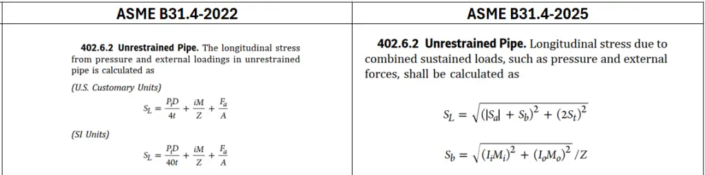
Updates in ASME B31.3 (2024) and B31.1 (2024) Piping Codes
The ASME B31 Piping Code Series governs piping systems in industries ranging from power plants to petrochemical facilities. The latest revisions focus on fatigue behavior, flange integrity, and nonlinear stress effects.
1. Fatigue and Stress Range Revisions
A key difference between the piping codes now exists in fatigue curves:
- B31.3 fatigue slope: −0.333
- B31.1 fatigue slope: −0.2
A steeper slope means B31.3 predicts fatigue damage more aggressively, particularly for high-cycle loading scenarios.
While future revisions may align these values, designers must currently account for the differences when working across both codes.
2. Expansion vs Occasional Loads
Clarification has been added to distinguish:
- Expansion stresses (thermal growth cycles)
- Occasional loads (seismic events, wind, relief loads)
For seismic design in particular, the code clarifies cycle counting considerations for repeated events.
This is important when performing fatigue screening during piping stress analysis.
3. Branch Connection Stress Intensification
Work continues to refine Stress Intensification Factors (SIFs) for branch connections.
Key trends include:
- Recognition that pressure stresses interact with bending stresses
- Greater reliance on finite element analysis (FEA) to validate SIF relationships
- Improved modeling of reinforcement pad behavior
As a result, many organizations are incorporating advanced stress modeling rather than relying solely on tabulated SIF values.
4. Flange Evaluation and Bolt Stress
The B31.3 code now explicitly recognizes that initial bolt-up stresses can exceed allowable stress limits during assembly.
This reflects real-world conditions where:
- Bolt preload is required to achieve sealing
- Relaxation and thermal effects reduce stresses during operation
Additionally, the draft ASME B31E Standard for Seismic Evaluation of Piping Systems introduces clearer criteria for distinguishing:
- Flange leakage
- Structural flange collapse
5. Recognition of Nonlinear Effects
Modern piping analysis increasingly considers nonlinear structural effects, including:
- Ratcheting
- Creep damage
- Local buckling
These phenomena are already addressed in Division 2 pressure vessel design and are now beginning to influence piping code philosophy.
Designers are encouraged to apply screening methods followed by advanced nonlinear analysis where necessary.
Updates in ASME Section IX-2025 (Welding and Brazing Qualifications)
The latest revision of Section IX includes several important changes to welding qualification procedures.
1. P-Number Revisions
Material grouping updates include:
- Removal of P-Number 49
- Addition of P-Number 81
These updates reflect the introduction of new alloys and changes in material classification.
Brazing P-Number tables have also been expanded, improving clarity for procedure qualification ranges.
2. Clarifications to Essential Variables
Several essential variables have been revised for clarity:
- QW-403.16 – Tube diameter qualification limits
- QW-403.32 – Wall thickness variables
These changes help remove ambiguity when qualifying welding procedures for small diameter piping and tubing systems.
3. New Variable for Wide-Weave Welding
A new essential variable has been introduced:
This variable addresses bead width and heat input control for wide-weave welding techniques.
Wide-weave welds can significantly influence heat input, residual stresses, and weld properties.
The addition of this variable ensures that heat input is properly controlled during welding procedure qualification.
Updates in AWS D1.1-2025
The AWS D1.1 Structural Welding Code – Steel governs welding practices for structural steel construction. The 2025 revision includes substantial updates to welding procedures and fabrication requirements.
1. Prequalified WPS Table Restructuring
Former Table 5.1 has been reorganized into four separate process-specific tables:
- SMAW
- SAW
- GMAW
- FCAW/GMAW-Cored
This restructuring improves clarity and makes it easier for engineers and welding coordinators to identify applicable rules for each process.
2. New GMAW Amperage Limits
Minimum amperage requirements have been introduced for GMAW welding procedures.
These limits depend on:
- Wire diameter
- Welding position
- Base metal thickness
The objective is to prevent low heat input welds that may produce lack of fusion defects.
3. FCAW and GMAW-Cored Electrode Updates
Electrode diameter selection rules now consider:
- Base metal thickness
- Welding position
This change ensures that electrodes are properly sized to achieve adequate penetration and weld quality.
4. Fabrication and Thermal Control Updates
Several fabrication clauses have been expanded:
Clause 6: Preheat and interpass temperature must now be listed explicitly on the WPS.
Clause 7: Expanded rules covering:
- Preheat control
- Interpass temperature limits
- Post-weld heat treatment (PWHT)
These changes strengthen process control during welding operations.
5. Inspection and NDT Updates
Inspection requirements have been updated to align more closely with American Society for Nondestructive Testing standards.
Improvements include:
- Refined discontinuity acceptance criteria
- Clearer guidance for inspection methods
- Expanded nondestructive testing rules
6. Introduction of Type D Studs
A new stud classification has been added:
Type D studs
These studs are designed specifically for structural steel applications, expanding the range of stud welding options available to fabricators.
Practical Implications for Pressure Vessel and Piping Engineers
The 2024–2025 revisions introduce several important implications for engineers working with pressure vessels, piping systems, and welded structures.
1. Increased Use of Division 2 Methods
Designers should expect to consult Division 2 calculations more frequently, even when working primarily under Division 1 rules.
This reflects the industry’s gradual shift toward stress-based design methodologies.
2. Documentation and Procedure Updates
Paragraph renumbering, rewritten clauses, and new variables require engineers to:
- Update internal design procedures
- Revise calculation templates
- Modify specification references
Failure to update documentation may lead to code compliance gaps during audits or design reviews.
3. More Conservative Design Calculations
The revisions introduce more conservative approaches in several areas:
- External pressure calculations
- Conical shell design
- Flange stress evaluation
These changes enhance structural reliability and safety margins.
4. Need for Updated Engineering Software
Engineering tools such as:
- Finglow
- DesignCalcs
- Paulin Research Group analysis tools must be updated to reflect the revised equations and material properties.
Engineers should validate software outputs against the updated code provisions before applying them in design projects.
Final Thought
The 2024–2025 revisions to major pressure vessel, piping, and welding codes reflect the industry’s ongoing shift toward more analytical design methods, improved material data, and stricter fabrication controls.
For pressure vessel and piping engineers, these updates emphasize the importance of:
- Familiarity with Division 2 analytical methods
- Careful documentation and procedure updates
- Integration of advanced analysis tools such as finite element analysis
- Continuous training to stay aligned with evolving code requirements
As codes become more technically rigorous and interconnected, engineers who stay current with these changes will be better equipped to design safer, more reliable pressure equipment and piping systems across modern industrial facilities.
Free Webinar on 2024–2025 ASME B31.3, B31.1, Sec VIII, Sec IX, and AWS D1.1 Code Changes
Want to get more insights on the above subject? Then learn from industry experts by learning from the free webinar mentioned below:
Click here to enroll and enjoy the Free Webinar