The Y factor is a dimensionless coefficient used for calculating the required wall thickness (t) for thin-walled pipes under internal pressure. According to Equation 3a of ASME B31.3, for determining the design pipe thickness, the application of the Y factor results in a reduction in the calculated wall thickness. In this article, we will examine the significance of factor Y in pipe wall thickness calculations.
The equation for pipe wall thickness calculation as per ASME B31.3 is given as
ASME B31.3-(3a): t = P.D/[2.(SEW+PY)]
Where:
- t = minimum required pipe wall thickness (excluding corrosion allowance)
- P = internal design pressure
- D = outside diameter of the pipe
- S = allowable stress of the pipe material at design temperature
- E = quality factor (depending on pipe manufacturing method)
- Y = coefficient from B31.3
- W = Weld Joint Strength Reduction Factor
Significance of Y-Factor in Pipe Thickness Calculation Formula
From the above equation, we can understand and interpret the reasons for using the Y factor as follows:
Simplification of thickness calculation: Instead of applying the equation for thick-walled pressure vessels, a simplified approach with a correction factor is used.
Design optimization: Prevents overestimation of the required wall thickness, thereby reducing project costs while maintaining compliance with safety requirements.
The pipe thickness is calculated based on the Lame’s hoop stress equation:

According to this equation, the stress across the pipe wall is not uniformly distributed. Therefore, to simplify the calculation and compensate for the non-uniform stress distribution, the Y factor is introduced.
Typical Values of Y-Factor in ASME B31.3
The value of Y is determined based on empirical data, allowing for some initial yielding at elevated temperature ranges.
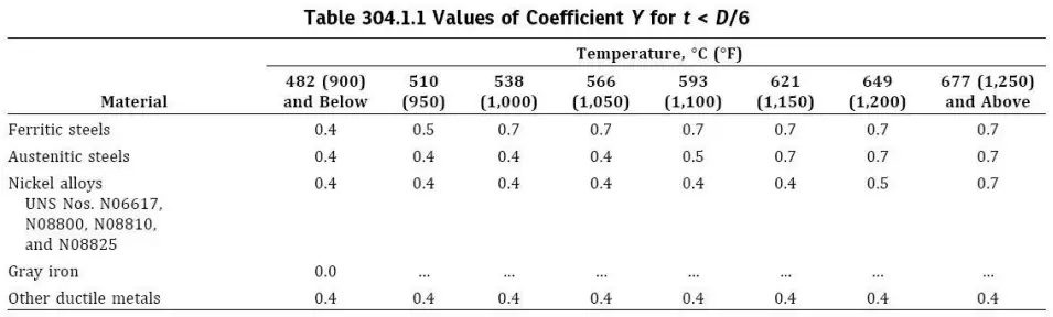
According to the provided table, an increase in temperature leads to an increase in the Y factor for certain materials. This implies that the code allows greater flexibility in thickness calculations at elevated temperatures, which is attributed to the material behavior under such conditions. A detailed explanation is provided below:
Based on Lame’s equation, the hoop stress is higher at the inner wall of the pipe compared to the outer wall, resulting in a non-uniform stress distribution. If wall thickness were calculated solely based on this equation, no Y factor would be applied, and the design would be based on the maximum hoop stress.
However, experimental observations have shown that localized yielding initially occurs at the inner wall of the pipe. This yielding does not lead to failure but instead allows for stress redistribution to other regions (e.g., the middle and outer wall). This process leads to a more uniform stress distribution across the pipe wall. As a result, the actual stress experienced by the pipe is lower than the peak value predicted by Lamé’s equation.
At higher temperatures, materials become softer, localized yielding occurs earlier, and the material naturally redistributes stress more effectively. Therefore, the code allows for a higher Y factor at elevated temperatures, acknowledging that the risk of stress concentration decreases due to improved stress distribution in softer material conditions.
It is important to note that for gray iron, the Y factor is specified as zero. This is because gray iron is brittle, has low tensile strength, and tends to fail suddenly without significant deformation. Due to its poor ability to absorb and redistribute localized stresses, the code adopts a conservative approach, not allowing any reduction in thickness through the Y factor.
For other ductile non-ferrous metals, the Y factor is constant across all temperatures. This is because such materials are already softer and more ductile than ferrous metals even at low temperatures. Therefore, localized yielding and stress redistribution occur early, and temperature increase does not significantly improve stress distribution. So, the code assigns a fixed Y value for all temperature ranges.
If the Y factor is not applied and the wall thickness is calculated based solely on the maximum hoop stress, the following consequences may occur:
- Increased material costs
- Greater complexity in welding and fabrication
- More challenging inspection and maintenance
- In most practical cases, economic efficiency is compromised without providing a meaningful increase in safety
References
- ASME B31.3 – Process Piping Code
- Pipe Stress Engineering – L.C. Peng and T.L. Peng