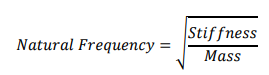
Natural frequency is determined by the physical properties of a piping system, like mass and stiffness, without any external driving force. This natural frequency in a piping system is affected by two major
factors which are as follows:
Rigidity vs Natural Frequency
Rigid piping systems exhibit a higher natural frequency. This rigidity can be the result of:
a. Pipe Size:
Higher size pipes or pipes with greater thickness are stiffer and naturally have higher frequencies, while smaller size pipes have lower natural frequencies. Even logically, a person cannot bend, deform, or move a large pipe easily, while they might be able to bend or move a ¾” pipe with ease.
b. Weight:
A piping system that contains water, compared to a piping system that contains gas, has more weight and cannot be easily moved or vibrated. In a sense, a much larger force and frequency are needed to create resonance and movement in a pipe filled with water than in a pipe filled with gas.
c. Number of Guide & Line Stop Support:
Naturally, a piping system that is restricted considerably cannot be easily moved or vibrated and exhibits a higher natural frequency. Because of the effect of pipe supports on the natural frequency, the piping system between every two supports can have a different natural frequency. This frequency can be different based on the distance between two supports, their types, pipe size, etc. So, in a piping system, a section might be moved and vibrate more easily, while another section, which has more support and is extremely rigid, cannot be easily moved or deformed.
Flexibility vs Natural Frequency
The more flexible a piping system is, the lower its natural frequency it has. In a sense, a flexible piping system can be easily moved or vibrated (This flexibility could be the result of size, fluid, and supports).
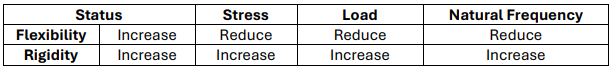
The best tool for a pipe stress engineer to reduce stress and load is to add more flexibility to the system. So, when we need to lower the stress and loads in a piping system, the best approach is to add flexibility to the system. The following table presents the relation between stress, load, flexibility, and rigidity in a piping system.
Resonance and Natural Frequency
Resonance vibration is a phenomenon occurring when an external force or vibrating system matches an object’s natural frequency, causing it to oscillate with significantly increased amplitude. It represents a state of maximum energy transfer, often resulting in amplified vibrations in mechanical, electrical, or acoustic systems.
So natural frequency becomes especially important in piping systems with a vibrating force, for example a reciprocating compressor or slug flow. If the frequency of the forced vibration matches the natural frequency of the system, the amplitude of the vibration will keep increasing, and will not be dampened which will eventually result in fatigue or large deformation and failure.
Important Notes in Natural Frequency Checking
When checking natural frequencies of a piping system, the following items become very important and
cause problems that will be explained one by one:
Frequency & Amplitude of Forced Vibration:
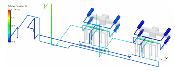
Even in a piping system that definitely has forced vibration like reciprocating compressors, checking natural frequency and increasing it to a significant number like 6Hz, which is common industry practice, and using vibration-damping support might not be enough, because the frequency of the forced vibration might actually be 6Hz. That is why the acoustic and vibration analysis of such systems is performed by the compressor vendor with consideration to the different frequencies of the compressor during start-up, normal operation, 20% above nominal speed, 50% nominal speed, etc. In many cases, the problem with vibration is fixed by adding vibration suppression devices or changing their size if they are already used (orifice plate or dampening capsule).
Pulsation study consists of using modeling techniques that account for the acoustic interactions between the compressor and piping. The modeling method must account for the dynamic interaction of flow through the valves and the dynamic pressure variation in the cylinder and in the cylinder passages immediately outside of the valves. Variations in specified operating conditions shall be analyzed by extending the analysis above and below the specified operating conditions. This is normally accomplished by simulating speeds above and below the specified speeds [API -618].
This vibration analysis may include passive piping analysis to determine the acoustic response of the piping. The piping system must be modeled to a point where the piping changes will have insignificant effects on the parts of the system under study (usually a large vessel upstream and downstream of the units to be studied) [API-618]. In a sense, a large volume acts as a pulsation dampening device, and after such a volume, there will no longer be a significant vibration effect in the system.
Off-Shore System on FPSO:
In FPSOs and topside platforms, the effects of green sea waves, sagging, hogging, etc., can adversely affect the life of the piping system, and because forced vibration is such a common aspect of these units, natural frequency and the life of a system under cyclic loads become extremely important. For such top-side process piping systems, there are specifications like DNVGL-RP-D-101 (Para 2.2.7.1), that ask for the frequency check above 4-5Hz to ensure safe operation of a piping system under constant movement of the ship due to waves and deformation of the ship due to sagging and hogging. In Top-side plants, in
addition to the natural frequency check, the cumulative fatigue life of the piping system and equipment must also be checked.
Two-Phase Flow:
There are various two-phase flow patterns in piping systems, but only the intermittent type of two-phase flow can cause vibration in a piping system [Applied Process Design for Chemical and Petrochemical Plants, Vol. 2, 3rd Ed., Ernest E. Ludwig].
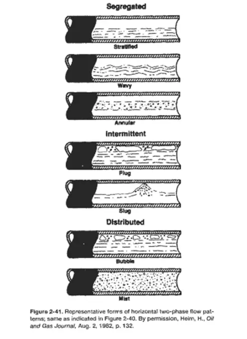
In the case of slug and plug flow patterns, the common industry practice is to add Reynolds force on elbows and make sure the stress within the piping system and its supports are below the allowable, and to check the natural frequency of the piping system to be above 3-4 Hz. This number may differ based on country, national standard, project specification, etc.
Vortex Shedding:
In subsea piping systems, the movement of seawater around the piping system
can cause vibrations due to vortex shedding (the same can happen for Wind). Vortex shedding is an unsteady flow phenomenon where alternating vortices detach from opposite sides of a bluff body (like a cylinder) in a fluid flow, creating a low-pressure wake.
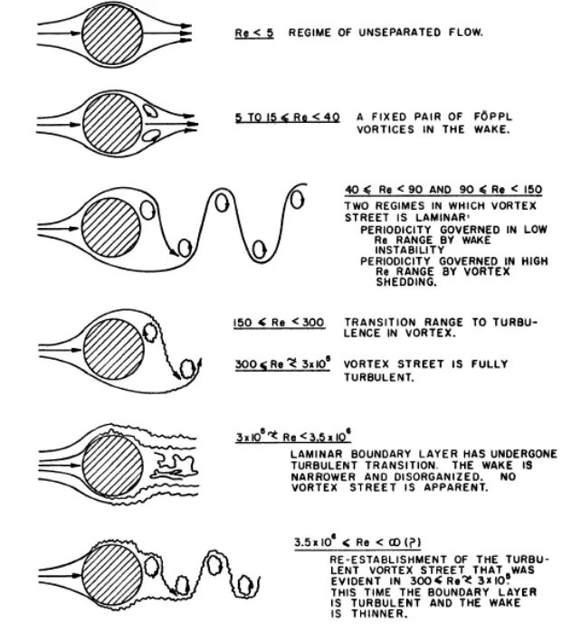
This phenomenon can cause vibration in sub-sea & riser piping system which need to be analyzed and checked for natural frequency and resonance possibility.
Common Client Requests and Their Challenges
In many projects, Clients believe a more rigid piping system is safer and less prone to vibration. They
usually request the natural frequencies of piping systems to be above 3 or 4 Hz in all cases and all piping systems without any consideration of the existence of a vibrating force.
1. Since most piping systems have no factor to cause vibration in them, checking this high natural frequency will lead to adding more support, guides, and stops to all piping systems, and lead to an overall increase in costs. Due to a lack of vibrating force, this is money spent on something that has no chance of happening.
2. Increasing natural frequency in a piping system will lead to increased rigidity in the system, and since this is opposite to flexibility, it complicates stress analysis of all piping systems. Since this checking is being done on all stress analysis files, it will result in more man-hours being spent on piping design, and in many cases, stress engineers will design systems with higher stresses and exert more loads on the adjacent equipment in order to satisfy the natural frequencies requested.
3. There are sections of piping systems, like expansion loops, that are inherently flexible and have low natural frequency. Fixing the natural frequency in expansion loops is either outright impossible or, in most cases, will result in unnatural piping designs/supports that are unacceptable to most Clients.
4. Small-diameter piping systems are flexible, and they usually exhibit low natural frequency. To fix this, a stress/support engineer has to add many pipe supports, and the final design may look unnatural. For example, it is not considered a clever design for a 2” piping system with a support every 3-4 meters to keep the natural frequency above 4 Hz.
5. Considering a high number like 4 Hz for all piping systems is extremely conservative and is usually considered for piping systems that have vibrating force in them, like slug flow. Designing all piping systems as if they have vibrations is not recommended.
Conclusion & Considerations
In the end, natural frequency is a complex matter to check in a piping system, and it can lead to profound changes in the design of the piping system, increase structural loads, and impose higher loads on connected equipment. It is highly recommended to check this phenomenon in the systems that actually undergo forced vibration and cyclic loading.
But if the client is persistent on checking the natural frequency on systems that have no forced vibration, extensive negotiations should be made to persuade them otherwise and the most logical compromise is to only check natural frequency near the equipment which actually cause vibrate like compressors, pumps (rotary equipment in general can cause local vibration in their vicinity), but should not be aggressively pursued since the allowable loads on these equipment are very sensitive and it is more important than a vibration with low chance of occurrence or high chance of getting damped in the first 10 meters of piping.
Also, selecting a high natural frequency as the goal can lead to unrealistic designs, and a reasonable amount should be selected for checking the natural frequency. An attempt should be made to negotiate a lower amount with the client.
In my opinion, the judgment of the pipe stress engineer in such matters is extremely important and should be highlighted. I strongly suggest leaving room for stress engineers to decide what is more important (higher natural frequency, lower stress, lower nozzle load, lower leakage percentage, or lower
support load) and allow them to optimize the piping system based on the thing that matters most. Limiting all possible avenues will result in strange designs that are not preferred by the Client.
I would also note to my stress engineer colleagues that a system without any guide, stop or limiting support is not favorable and attempt should be made to restrict the movement of pipe and increasing its natural frequency, in case there is a water hammer due to emergency closure of a valve or forming slug flow during transient cases of start up or shut down or a major seismic activity.
Special Thanks to Mr. Javad Jahankhah for sharing this insight.