
Glass Reinforced Piping (GRP) products, being proprietary, the choice of component sizes, fittings, and material types are limited depending on the supplier. Potential GRP vendors need to be identified early in the design stage to determine possible limitations of component availability. The mechanical properties and design parameters vary from vendor to vendor. Note that the stress analysis methodologies of Fiber Reinforced Piping (FRP) and Glass Reinforced Epoxy (GRE) are similar and performed following the ISO 14692 code. As the design parameters are dependent on the manufacturers, it is of utmost importance that before you proceed with stress analysis of such systems you must finalize the GRP/FRP/GRE vendor.
Several parameters (Fig. 1) for stress analysis have to be taken from the vendor.
Stress analysis of the GRP piping system is governed by ISO 14692 part 3. The GRP material being orthotropic the stress values in axial as well as hoop direction need to be considered during analysis. The following article will provide a guideline for stress analysis of the GRP piping system in a very simple format.
GRP/FRP Information Required from Vendor
Before you open the input spreadsheet of Caesar II communicate with the vendor through the mail and collect the following parameters as listed in Fig.1.
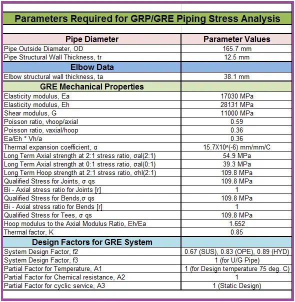
The values shown in the above figure are for example only. Actual values will differ from vendor to vendor. The above parameters are shown for a 6” pipe.
Inputs Required for GRP Stress Analysis
For performing the stress analysis of a GRP piping system following inputs are required:
- GRP pipe parameters as shown in Fig. 1.
- Pipe routing plan in the form of isometrics or piping GA.
- Analysis parameters like design temperature, design pressure, operating temperature, fluid density, hydro test pressure, pipe diameter, thickness, etc.
Modeling GRP/FRP/GRE in Caesar II
Once all inputs as mentioned above are ready with you open the Caesar II spreadsheet. By default, Caesar will show B31.3 as the governing code. Now refer to Fig. 2 and change the parameters as mentioned below:
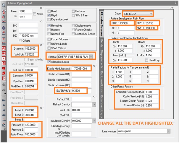
- Change the default code to ISO 14692.
- Change the material to FRP (Caesar Database Material Number 20) as shown in Fig. 2. It will fill a few parameters from Caesar’s database. Update those parameters from vendor information.
- Enter pipe OD and thickness from vendor information.
- Keep corrosion allowance as 0.
- Input T1, T2, P1, HP, and fluid density from the line list.
- Update pipe density from the vendor information sheet, if the vendor does not provide the density of the pipe then you can keep this value unchanged.
- On the right side below the code, enter the failure envelope data received from the vendor.
- Enter thermal factor=0.85 if the pipe is carrying liquid, and enter 0.8 if the pipe carries gas.
- After you have mentioned all the highlighted fields proceed to model by providing dimensions from the isometric/piping GA drawing. Add supports at the proper location from the isometric drawing.
- Now click on the environment button and then on the special execution parameter. It will open the window as mentioned in Figure 3.
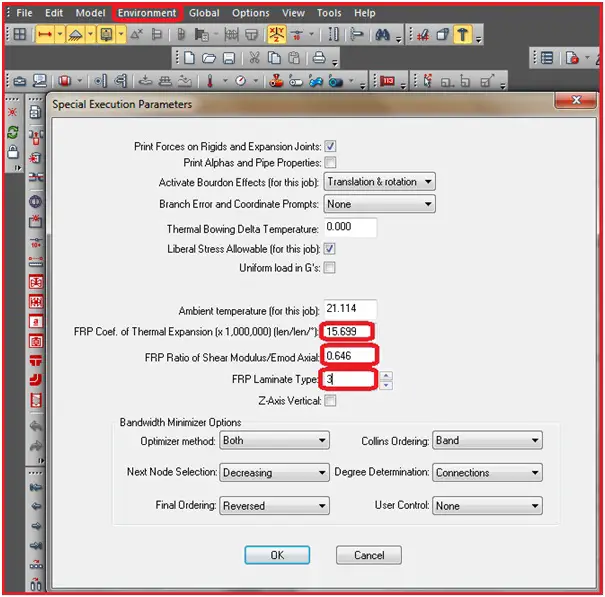
Now Refer to Fig. 3 and change the highlighted parts from the available data.
- Enter the GRP/FRP co-efficient of thermal expansion received from the vendor
- Calculate the ratio of Shear Modulus and Axial modulus and input in the location.
- In FRP laminate keep the default value if data is not available.
- After the above changes click on the ok button.
- While modeling, remember to change the OD and thickness of elbows/bends.
Modeling of GRE Bend and Tee Connections
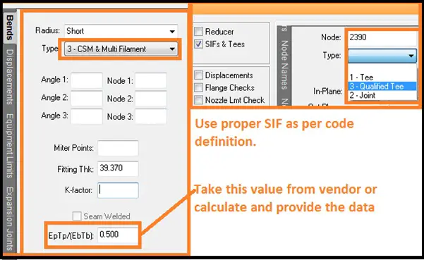
- The modeling of bends is a bit different as compared to CS piping. Normally, bend thicknesses are higher than the corresponding piping thickness. Additionally, you have to specify the parameter, (EpTp)/(EbTb), which is located at the Bend auxiliary dialogue box as shown in Fig. 4. This value affects the calculation of the flexibility factor for bends.
- When you click on the SIF and Tee box in the Caesar II spreadsheet, you will find that only three options (Tee, Joint, and Qualified Tee) are available for you, as shown in Fig. 4. Each type has its own code equation for SIF calculation. Use the proper connection judiciously. It is always better to use SIF as 2.3 for both inplane and outplane SIF to adopt a maximum conservative approach.
Stress Analysis Load Cases for FRP Piping Systems:
ISO 14692 informs to prepare 3 load cases: Sustained, Sustained with thermal, and Hydro test. So accordingly, the following load cases are sufficient to analyze the GRP piping system
- WW+HP …………………….HYDRO
- W+T1+P1 …………………..OPERATING-MAXIMUM DESIGN TEMPERATURE
- W+T2+P1 …………………..OPERATING-OPERATING TEMPERATURE
- W+T3+P1 …………………..OPERATING-MINIMUM DESIGN TEMPERATURE
- W+P1 ………………………..SUSTAINED
Here,
- WW: Water-filled weight
- HP=Hydrotest pressure
- T1=Maximum design temperature
- T2=Maximum operating temperature
- T3=Minimum design temperature
- P1=Design pressure, and
- W=Content filled pipe weight
The expansion load cases are not required to be created as no allowable stress is available for them as per the code.
Note that, sometimes GRE piping network may have slug scenarios when carrying two-phase liquids. Again, they may have surge scenarios like firewater GRE pipe networks. So, those forces, if any, need to be considered additionally, as the case may be.
Again, if you are analyzing a piping system consisting of GRE pipe plus metallic piping, then expansion load cases need to be prepared.
While preparing the above load cases you have to specify the occasional load factors for each load case in the load case options menu as shown in Fig. 5. ISO 14692 considers hydro test case as an occasional case. In higher versions of Caesar II software (Caesar II-2016 onwards), these load factors are taken care of by default. So you need not enter the values. The option of these value entries will be available only if you define the stress type as occasional for those software versions.
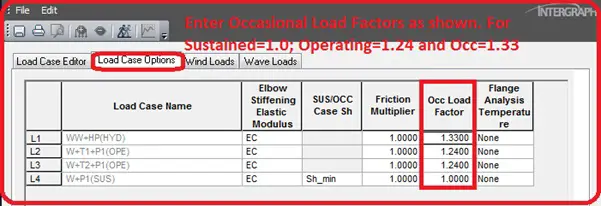
The default values of occasional load factors are 1.33 for the occasional case, 1.24 for the operating case, and 1.0 for the sustained case. These occasional load factors are multiplied with the system design factor (normally 0.67) to calculate the part factor for loading f2.
For aboveground GRP piping, the above load cases are sufficient. But if the line is laid underground, then two different Caesar II files are required. One for sustained and operating stress checks. The other is for hydro testing stress check as the buried depth during hydro testing is different from the original operation. Also, buried depth may vary in many places. So, Caesar II modeling should be done meticulously to take care of the exact effects.
For buried GRP pipe modeling, one needs to split the long lengths into shorter elements to get proper results. An element length of 3 m or less is advisable. Sometimes buried model contains a pipe slope, Those slopes are required to be modeled properly to get accurate results.
Code Stresses as per ISO 14692-2005
ISO 14692 2005 requires that the sum of all hoop stresses (σh, sum) and the sum of all axial stresses (σa, sum) be evaluated for all states of the piping system. CAESAR II evaluates these stresses for stress types OPE, SUS, and OCC. If the hoop stress is exceeded, the axial stress is not reported.
There are two stress envelopes in ISO 14692; Fully Measured Envelope and Simplified Envelope.
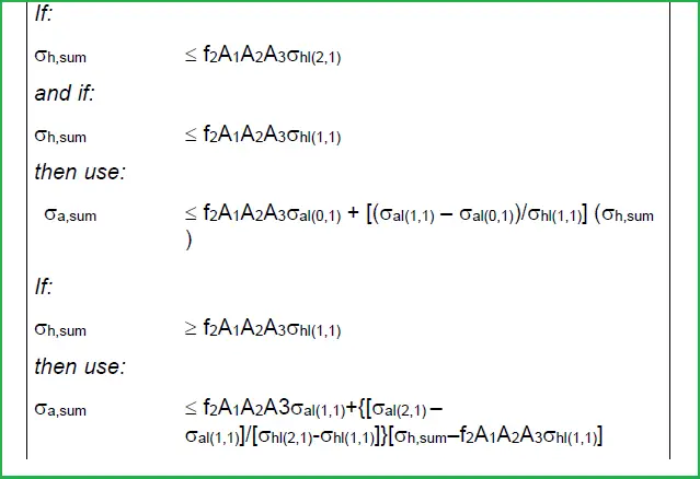
Stress Equations as per the Fully Measured Envelope
For Fully Measured Envelope; the inputs of σhl(1,1) and σal(1,1) are required in the piping input spreadsheet. The equations used in Caesar II software when analyzing using a fully measured envelope are as follows:
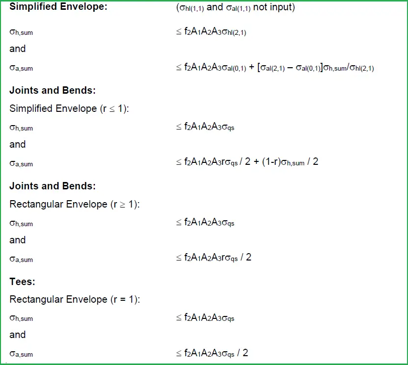
Stress Equations as per the Simplified Envelope
For Simplified Envelope, the inputs of σhl(1,1) and σal(1,1) are not required in the piping input spreadsheet. The equations used in Caesar II software when analyzing using a simplified envelope are as follows:
Explanation of the symbols used in the above equations:
The significance of the symbols that are used in the above-mentioned equations are:
- f2 = Part Factor for Loading
- 0.89 for Occasional Short-Term Loads
- 0.83 for Sustained Loads Including Thermal Loads
- 0.67 for Sustained Loads Excluding Thermal Loads
- A1 = Partial Factor for Temperature
- A2 = Partial Factor for Chemical Resistance
- A3 = Partial Factor for Cyclic Service
- σqs = Qualified Stress (entered for bends, fittings, and joints)
- σal(0,1) = Long-Term Axial Strength at 0:1 Stress Ratio
- σal(1,1) = Long-Term Axial Strength at 1:1 Stress Ratio
- σhl(1,1) = Long-Term Hoop Strength at 1:1 Stress Ratio
- σal(2,1) = Long-Term Axial Strength at 2:1 Stress Ratio
- σhl(2,1) = Long-Term Hoop Strength at 2:1 Stress Ratio
- r = Bi-Axial Stress Ratio 2σal(0,1)/σqs (for simplified and rectangular envelopes)
- σa,sum = Sum of All Axial Stresses {(σap + σab)2 + 4ξ2}1/2
- σh,sum = Sum of All Hoop Stresses [σh2 + 4ξ2]1/2
- σap = Axial Pressure Stress
- σab = Axial Bending Stress
- ξ = Torsion Stress
- σh = Hoop Stress
Note that, in the year 2017, ISO 14692 received a new update, and there are many changes, which are explained here: What’s new in ISO 14692-2017?
Output Results from GRP Stress Analysis
Both stress and load data need to be checked for GRP piping. Normally the stresses are more than 90% (Even, sometimes it may be as high as 99.9%).
Few more related articles for you.
Stress Analysis of GRP / GRE / FRP Piping using START-PROF
What’s new in Revised ISO 14692: 2017 Edition
HYDROSTATIC FIELD TEST of GRP / GRE lines
Stress Analysis of GRP / GRE / FRP piping system using Caesar II
A short article on GRP Pipe for beginners
Online Video Course on FRP Pipe Stress Analysis
I have prepared a dedicated online course for explaining the steps followed in FRP/GRP/GRE pipe stress analysis using Caesar II.
Very good article.
Thanks.
Interesting article, can u please explain which wall thickness i should take in Caesar II input (the total wall thickness or the reinforced thickness) waiting for your second part. Thanks
please post part 2
Anup very nice presentation.. Excellent useful article!!
So useful article. would you please explain how can i simulate the vibration condition pump discharge in CAESAR II in the GRP Piping?
nice article,pl provide the second part of it also
Hai sir I am a piping engineer I am working in abudhabi ADNOC plant , your article very clear and easy to understand ,thank you
If we have Wind and earthquake. How did we define load combinations and stress type in this cases ?
Thank you for procedure. But what if we wanted conduct fatigue analysis on it.
you haven’t mentioned anywhere in the article!
Very Good article! It helps me a lot. But now we will use the ISO 14692-2017 for GRE Piping System. Looking forward to your update.