Advantages of using Coordinate System in Caesar II

As Pipe Stress Engineers, we all, in some way or other, have handled the assignment of modeling and analyzing parallel lines routed over pipe racks or sleepers. Often these lines require Expansion Loops to have sufficient flexibility. However, although may be routed kilometers, these lines often do not have any interconnection between them. Therefore, normal practice is to model these lines in separate ‘.C2’ files and carry out stress analysis and expansion loops sizing and positioning separately. Now, suppose if we could model all lines running parallel to each other in a corridor and with the same design code (e.g. B31.3) in a single ‘.C2’ file, then not only we could view and review all the lines together, but also we could size and locate expansion loops for each line with respect to the others. This would not only reduce the modeling and analysis efforts but would also enable us to handle a lesser number of CAESAR II native files.

This is pretty well possible with the help of the ‘Block Operation’ and ‘Coordinate’ features in CAESAR II. In my earlier post titled “ADVANTAGE OF USING ‘BLOCK OPERATION’ IN CAESAR II, “ I tried to explain ‘Block Operation’. In this post, I would attempt to highlight the effective use of the ‘Coordinate’ feature.

Let us take the case of two lines running parallel to each other over a Pipe Rack, and supported in the same locations.

Parameters for Line 1:

• Design Code = ASME B31.3
• MOC = ASTM A106 Gr. B
• Size = 12”
• Sch. = STD
• Corrosion Allowance = 1.5 mm
• Design Pressure = 1200 kPa(g)
• Design Temperature = 175^OC
• Fluid Density = 900 kg/m³
• Insulation = Mineral Wool
• Insulation Thickness = 50 mm
• Cladding Thickness = 0.7 mm
• Cladding Density (Aluminium) = 2700 kg/m³

Parameters for Line 2:

• Design Code = ASME B31.3
• MOC = ASTM A106 Gr. B
• Size = 10”
• Sch. = STD
• Corrosion Allowance = 1.5 mm
• Design Pressure = 1800 kPa(g)
• Design Temperature = 150^OC
• Fluid Density = 900 kg/m³
• Insulation = Mineral Wool
• Insulation Thickness = 50 mm
• Cladding Thickness = 0.7 mm
• Cladding Density (Aluminium) = 2700 kg/m³

Let us assume these two lines are having a gap of 500 mm between centerlines.

First, we model Line 1 as per the given parameters.

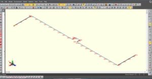
Line 1 starts at Node 10 and ends at Node 370.

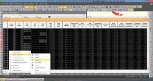
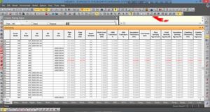
Now, we invoke ‘List Input’.

Then, at the ‘List Input’ window, we select all elements, right-click, select ‘Block Operation’ and then select ‘Duplicate’.

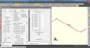
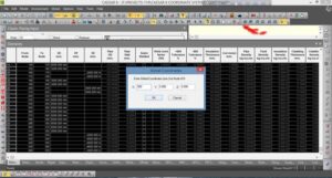
In the ‘Block Duplicate’ window, under the ‘Options’ tab, we select ‘Identical’, under the ‘Insert Copied Block’ tab, we select ‘At End of Input’, and input ‘400’ in the ‘Node Increment’ box, and click ‘OK’.

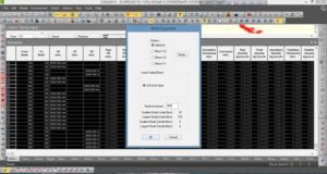
Now, we input ‘500’ in the box of X coordinate in ‘Enter Global Coordinates (mm.) for Node 410’ under the ‘Global Coordinates’ window.

Now, we have created the geometry of Line 2, but still with the parameters of Line 1. So, we change the parameters as applicable.

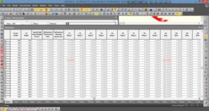
Then, we close the ‘List Input’ window.

Now, we are ready with two lines that are running in the same route, supported at the same locations, but still requiring some manual modifications at the elbows of Line 2.

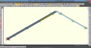
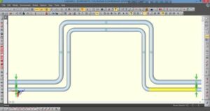
So, we reduce the lengths of elements before and after the first elbow by 500 mm. Likewise, we adjust the expansion loop of Line 2 to arrive at the following geometry in Figure – 9.

Finally, we increase the lengths of elements before and after the last elbow by 500 mm.

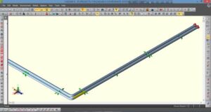
This completes the parametric and geometric adjustments of Line 2.

Now, both of the lines are ready for onward analysis.

Note: Although this is a useful and smart way of working, the stress analyst must use his/her judgment for use of this feature, particularly if the lines are to be analyzed under different codes, it is recommended not to use this feature. Also, the model shown as an example is a very simplified one. An analyst may encounter more complex problems, and the extent of manual adjustment is likely to vary from little to more on a case-by-case basis.