This post is solely for beginners in the piping industry. If you want to learn the basics from books or literature, then try the following 15 listed books. Most experienced piping professionals will be aware of these piping books. Most of the piping books and literature mentioned below are available for free downloading over the internet. Simply search with the book name along with the term pdf, and you will get it. All these piping engineering books are also available in the Amazon online portal, from where you can easily buy them. Additionally, simply do an exclusive search on the internet, and you will find some links to download these piping books for free.
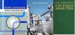
1. PIPE STRESS ENGINEERING by L C Peng and T L Peng:
This is the best book on piping stress engineering. If you are planning a career in piping stress analysis, then you must collect this book and read it effectively to build solid basics. This book explains the ideas so nicely that it will provide effective results to you.
It delves deeply into the principles and methodologies of pipe stress analysis. The book offers an extensive exploration of stress analysis techniques, focusing on the mechanical behavior of pipes under various loads and conditions. It covers critical topics such as thermal expansion, pipe supports, and the impacts of different loading scenarios on pipe integrity. Detailed explanations are provided on methods for calculating stress, evaluating pipe supports, and designing systems to manage stress-related issues. The inclusion of practical case studies and real-world examples further enriches the content, illustrating how theoretical principles are applied in practice.
What sets Peng’s book apart as a premier resource for pipe stress engineers is its comprehensive and practical approach to a complex subject. The authors’ ability to break down intricate concepts into understandable segments makes this book invaluable for both seasoned professionals and those new to the field. The practical guidance on managing stress-related issues and the integration of case studies provide actionable insights that are directly applicable to everyday engineering challenges. The book’s focus on real-world applications and problem-solving ensures that it remains a crucial reference for engineers aiming to enhance their expertise in pipe stress engineering and ensure the reliability and safety of their piping systems.
2. DESIGN OF PIPING SYSTEMS by M W Kellogg Company:
This is the second-best book on piping stress analysis. Even though the language used is quite difficult to comprehend and the contents are not interesting, this book shares a great place for describing the topics effectively and was the best book earlier before the Peng book.
M. W. Kellogg’s “Design of Piping Systems” is a classic text that provides a detailed examination of the principles and practices involved in designing piping systems. The book covers a range of topics including pipe sizing, stress analysis, and material selection. Kellogg’s text is known for its depth of coverage and its methodical approach to addressing the various challenges encountered in piping system design. It also includes practical examples and case studies to illustrate key concepts.
The enduring relevance of Kellogg’s book lies in its thorough and systematic approach to piping system design. The book’s detailed explanations and comprehensive coverage make it a valuable reference for engineers seeking a deep understanding of piping design principles. Its combination of theoretical knowledge and practical examples ensures that it remains a key resource for both learning and applying piping design techniques.
3. INTRODUCTION TO PIPE STRESS ANALYSIS by Sam Kannapan:
One of the best books on piping stress analysis and is easy to understand. “Introduction to Pipe Stress Analysis” by Sam Kannapan is an accessible yet thorough guide designed to introduce engineers to the principles and practices of pipe stress analysis. This book covers fundamental concepts such as the behavior of pipes under various loading conditions, stress calculation methods, and the importance of proper pipe support and restraint systems. Kannapan provides a clear explanation of key topics including thermal expansion, pipe flexibility, and the impact of different types of loads on pipe systems. The book is structured to build a solid foundation in pipe stress analysis through clear illustrations, examples, and straightforward explanations.
The strength of Kannapan’s book lies in its approachability and clarity, making it an ideal resource for both newcomers and seasoned engineers seeking a refresher. The practical focus and structured presentation of complex concepts makes it easier for readers to grasp and apply pipe stress analysis principles in real-world scenarios. The book’s emphasis on fundamental techniques, combined with practical examples and problem-solving strategies, ensures that it serves as an excellent reference for engineers aiming to understand and address stress-related challenges in piping systems effectively.
4. COADE STRESS ANALYSIS SEMINAR NOTES by COADE:
Must have a tutorial guide for every piping stress engineer using CAESAR II. Explains in detail all the basics of Caesar II’s application. The guidebook is developed by Hexagon (COADE) and explains all the basic concepts that are used for the development of the Caesar II software program.
5. PIPING HANDBOOK by M L Nayyar:
One good book for both stress and layout engineers with the huge important databases on piping engineering. Refer to this book for any data you require during your day-to-day piping work. The “Piping Handbook” by Mohinder L. Nayyar is a definitive resource that encompasses a wide array of topics essential for piping engineers. This book covers everything from basic piping design principles to advanced topics such as pipe stress analysis, hydraulic calculations, and material properties. Nayyar’s handbook is renowned for its detailed tables, charts, and formulas that aid in the design and analysis of piping systems. It also addresses various industry codes and standards, providing a thorough grounding in compliance and best practices.
What makes Nayyar’s Piping Handbook an excellent reference is its broad scope and depth of coverage. The book’s extensive collection of practical data and guidance makes it a useful tool for engineers working in diverse industries, from oil and gas to chemical processing. Its emphasis on real-world applications and problem-solving, combined with its comprehensive coverage of standards and regulations, ensures that it remains a critical resource for professionals seeking reliable and detailed information.
6. PIPE DRAFTING AND DESIGN by Rhea and Perisher:
The best book for a beginner. Covers the basics in simple language. Very easy to understand. “Pipe Drafting and Design” by Rhea and Perisher is a comprehensive guide that provides a detailed overview of the principles and practices involved in drafting and designing piping systems. The book covers a wide range of basic topics, including the fundamentals of pipe drafting, design standards, and the various types of piping systems used in different industries. Rhea and Perisher delve into the technical aspects of piping design, such as pipe layout, the selection of materials, and the application of industry codes and standards. The text also emphasizes the use of drafting software and tools, making it relevant for modern design practices.
This book is highly regarded for its practical approach and its ability to bridge the gap between theoretical knowledge and real-world drafting application. Rhea and Perisher’s clear explanations and step-by-step guidance make complex design concepts more accessible, helping both novice and experienced engineers enhance their drafting and design skills. The inclusion of detailed illustrations, case studies, and practical examples provides valuable insights into the design process, making it a valuable reference for anyone involved in the drafting and design of piping systems. Its focus on both traditional techniques and modern tools ensures that it remains relevant in today’s evolving engineering landscape.
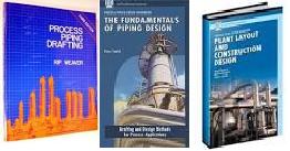
7. PROCESS PLANT LAYOUT AND PIPING DESIGN by Hunt and Bausbacher:
The best book for a piping layout engineer. Covers the basics of the piping layout. Most of the preliminary layout ideas connected to any equipment evolve from this book. So read this book attentively for effective layout knowledge.
“Process Plant Layout and Piping Design” by Ed Bausbacher and Roger Hunt is a highly regarded text that provides an in-depth exploration of the principles and practices involved in the layout and design of piping systems in process plants. The book covers a wide range of topics essential for effective process plant design, including the fundamentals of layout planning, equipment arrangement, and the integration of piping systems with plant processes. Bausbacher and Hunt address critical considerations such as safety, accessibility, and efficiency in piping design, offering practical guidelines for optimizing plant layout and ensuring operational effectiveness.
The value of this book lies in its comprehensive and practical approach to process plant layout and piping design. Bausbacher and Hunt’s expertise is evident in their detailed explanations and real-world examples, which help readers understand complex design concepts and apply them to practical situations. The book’s focus on optimizing plant layouts for safety and efficiency makes it an essential resource for engineers involved in the design and operation of process plants. Its combination of theoretical knowledge and practical application ensures that it remains a crucial reference for achieving effective and efficient process plant design.
8. PROCESS PIPING DESIGN HANDBOOK by John Mcketta:
One of the good books. The “Process Piping Design Handbook” by John J. McKetta Jr. focuses on the detailed aspects of designing piping systems specifically for process industries. McKetta’s handbook covers various design considerations such as flow dynamics, material selection, and the integration of piping with process equipment. It provides in-depth guidance on designing for safety, reliability, and efficiency, addressing issues such as thermal and mechanical stresses, as well as corrosion control.
McKetta’s handbook is highly valued for its targeted focus on process piping, making it an essential resource for engineers working in process industries. The book’s detailed coverage of design principles and its emphasis on practical design considerations ensure that it provides relevant and applicable knowledge for engineers looking to optimize their process piping systems. Its thorough exploration of industry-specific challenges and solutions enhances its utility as a reference for both design and troubleshooting.
9. THE FUNDAMENTALS OF PIPING DESIGN by Peter Smith
Peter Smith’s “Fundamentals of Piping Design” is an accessible yet comprehensive introduction to the principles and practices of piping design. The book covers fundamental topics such as system layout, pipe sizing, and material selection. Smith’s approach is designed to build a solid foundation in piping design, making complex concepts understandable for newcomers while providing enough depth to be valuable to experienced engineers. It also includes practical design examples and problems to reinforce the learning experience.
The strength of Smith’s book lies in its clear and methodical approach to piping design fundamentals. It provides a structured pathway for learning the basics of piping design, making it an excellent resource for engineers new to the field or those seeking to refresh their knowledge. Its emphasis on practical examples and clear explanations makes it a valuable tool for developing a strong understanding of piping design principles and practices.
10. “PIPING AND PIPELINE ENGINEERING” by George A. Antaki
“Piping and Pipeline Engineering” by George A. Antaki is a comprehensive guide that covers all critical aspects of piping and pipeline design and maintenance. The book delves into the fundamental principles of fluid dynamics, materials selection, and the mechanical aspects of pipeline systems. Antaki’s text is structured to provide both theoretical knowledge and practical insights, making it an invaluable resource for understanding the lifecycle of piping systems from design through construction and maintenance. It includes detailed coverage of pipe stress analysis, corrosion, and inspection techniques.
This book stands out as a top reference for piping engineers due to its extensive scope and clarity. Antaki’s approach integrates real-world scenarios with theoretical concepts, offering practical solutions to common issues encountered in the field. The inclusion of case studies and practical examples helps bridge the gap between theory and practice, making it a go-to resource for both novice and experienced engineers seeking to deepen their understanding of piping systems.
Other Notable Piping Books
Some other notable piping books that readers can keep as a reference book are:
- 11. PROCESS PIPING DRAFTING By Rip Weaver: A very nice book in simple, easy-to-understandable language.
- 12. THE PLANNING GUIDE TO PIPING DESIGN by Richard Beale
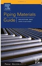
- 13. One must-have book for piping materials engineers is PIPING MATERIALS GUIDE by Peter Smith
- 14. PIPING SYSTEMS MANUAL by Brian Silowash
- 15. PIPING DESIGN FOR PROCESS PLANTS by Rase Howard F
In addition to all the above-mentioned piping books, you must remember that you have to read the latest applicable piping codes as well.
All of You are already aware that books are our best friends. It helps us without charging us. So enjoy reading.