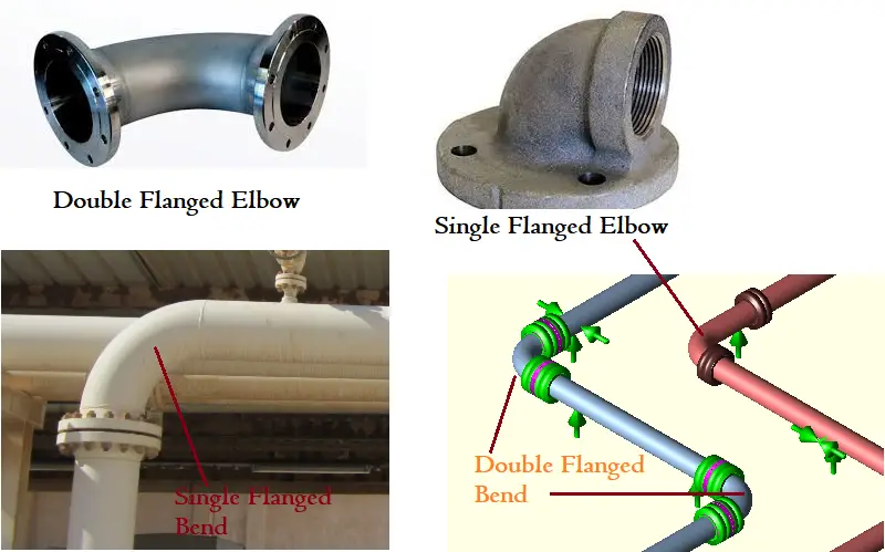
Flanged pipe bends or flanged elbows are piping elbows connected with flange fitting to fitting. This means there is no spool or pipe piece in between the elbow endpoint( weld point) and flange. Flanged elbows are widely used for piping connections requiring compact pipe routing. Flanged elbows are purchased as a pipe fitting. On the other hand, flanged bends are prepared when a flange (weld neck or any other type) is directly welded to a piping elbow.
Types of Flanged Elbows
Based on the number of flanges connected to the pipe elbow fitting, flanged bends are of two types:
Single Flanged Elbow and
Double Flanged Elbow
When one side of a pipe elbow is connected to a flange but the other side is connected to a pipe it is called a single-flanged elbow. Again when there are flanges on both sides of the elbows, it is called a double-flanged elbow. Refer to Fig. 1 for a typical example.
Fig. 1: Single and Double Flanged Elbow
Effect of Flanged Elbow or Flanged Bend
When the flanges are attached near elbows or bends (Near Control Valve assembly and equipment nozzles); they exert a severe restraining force on the flexibility of the bend, thus reducing the flexibility of the bend and increasing the force and moment in the nearby support or nozzle. ASME B 31.3/ASME B31J Code provides two correction factors C1 and C2 to take care of the same effect. So basically the single-flange and double-flange options provide the following impacts in a piping system:
In Caesar II software the effect of the flanged bend can be easily taken care of by modeling flanged elbows as mentioned below.
Sometimes dummy/trunnion attachments at the elbow also provide a similar effect which is why a few organizations have the practice of using a flanged elbow while modeling the trunnions from the elbow.
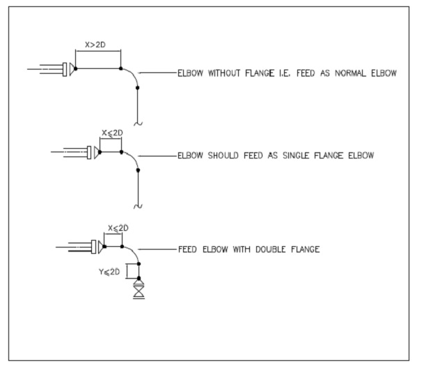
Single or Double Flange Option should be applied to Stress Analysis if there is any flanges or valves (heavy/rigid body) within two diameters (2D as per BS 806) of the ending weld point of the bend as shown in Fig. 2.
Fig. 2: Criteria for using Flanged Bend in Caesar II
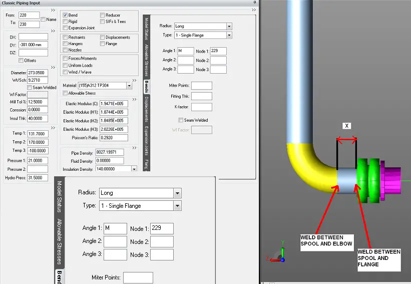
The modeling steps for the flanged bend are shown in Fig. 3. Single flanged bend is indicated by selecting 1-Single Flange as shown in Fig. 3. Similarly Double Flanged Bend can be indicated by selecting the 2-Double Flange option.
Fig. 3: Caesar model showing the flanged bend application criteria
What if Piping Continuation is Unknown? Part 1. Above Ground Piping
What if Above Ground Piping Continuation is Unknown?
The correct model and boundary conditions are very important for accurate piping stress analysis. Unfortunately, some inexperienced piping stress analysis software users made mistakes caused by lack of knowledge in structural mechanics.
Incorrect boundary conditions at the points where piping continuation is unknown is the most common mistake. It happens when other parts of the piping are designed by other companies or departments. Sometimes the design of these parts is not finished or even started. In this case some engineers create the incorrect piping stress models like shown below. It is the piping model in which some of the ends are free and don’t contain any restraints (nodes А, В, С, D, E, F). Free ends – is fictional border between “our” and “other” piping parts. In reality the piping continues after these points. The models below was sent to the PASS/START-PROF technical support by some of our customers.
These models are totally wrong, because the boundary conditions allow piping to expand freely. The stresses, support loads become a very low. But this is just an illusion.
Such models are totally wrong because its behavior and behavior of real piping is completely different. Nodes А, В, С, D, E, F can freely move due to temperature expansion. The stresses and support loads in this model will be much smaller than in real piping.
Let’s see the difference in results on the example shown below. Pipe 219×6, pressure 1.6 MPa, steel 20, temperature 200 C. Anchor is placed in at node 2, U-shaped loop (5-4), and the continuation after node 3 is unknown.
Model 1
If we cut piping at node 3 – we will get anchor (node 2) load 653.1 kgf, the stresses satisfy the code requirements.
Model 2
After we place an anchor in node 3 the anchor (node 2) load is much greater – 2153 kgf. Stresses are still satisfying the code requirements. The anchor or hinged anchor in node 3 gives us the safety margin comparing to the previous example. But sometimes the safety margin is not enough, see the “model 4” example.
Model 3
Let’s model one of possible variants of piping model after node 3. It’s L-shaped loop. The support load is lower than in previous example (model 2) but higher than in model 1 – 809 kgf.
Model 4
It is the worst case. After node 3 is a long straight pipe. The support (node 2) load is greatest – 3074 kgf. Also the stresses are higher than allowable. Model 4 is the worst because the straight pipe 35-3 doesn’t have any expansion loops and it push the point 16 from the right to left.
Conclusion
The piping design after the fictional border (node 3) influences the results very high. That’s because the most accurate results can be obtained only if we model the whole piping, not just a part of piping.
In case if it’s impossible, it is recommended to place the Anchor, Hinged Anchor or Line Stop in fictional end point (node 3).
Hinged anchor used in START-PROF software. In other software it is modeled as combination of Rest, Guide, and Axial Stop restraints. Hinged Anchor gives us the greatest safety margin, because it stops the temperature expansion, and allows pipe rotation under weight loads.
Possible options in this situation:
Model the whole piping. But sometimes it’s impossible because the continuation is unknown
Model the part of piping. All fictional border points should be modeled as anchors or hinged anchors. Also just Line Stop restraint could be used in some cases. This model will give additional safety margin, but this margin could not be enough in some situations. Usually this model is used for piping
Model the part of piping and add the virtual straight pipes at the points A, B, C, D, E, F. Or add anchors in points A, B, C, D, E, F with movement. This modeling technique is usually used to take into account the possible temperature expansion of connected long above ground pipelines
What is a Pressure Gauge? Types of Pressure Measuring Instruments
Pressure Gauges are pressure measuring instruments. Pressure and Temperature are two very important parameters for all chemical industries. So, pressure measurement is of utmost importance. There are various pressure-measuring instruments available to perform this task. Pressure measurement basically means the analysis of the fluid forces that are imparted on a surface. The accuracy of pressure-measuring instruments is very important for proper operational control. In this article, we will explore various pressure measuring devices or pressure gauges used across industries.
What is a Pressure Gauge?
A pressure gauge is a device used to measure the pressure of a fluid or gas in a closed system. It typically consists of a Bourdon tube, which is a curved tube that is connected to the system being measured. When the pressure inside the system changes, the Bourdon tube flexes and moves a pointer on a dial, indicating the pressure reading.
Pressure gauges are used in a wide range of applications, including industrial processes, heating and cooling systems, automotive and aerospace systems, and medical devices. They come in various sizes, types, and accuracy levels, and can measure different units of pressure such as psi (pounds per square inch), kPa (kiloPascals), bar, and mmHg (millimeters of mercury).
Proper calibration and maintenance of pressure gauges are important to ensure accurate and reliable readings. Depending on the application, pressure gauges may need to meet specific industry standards and regulations, such as those set by the American Society of Mechanical Engineers (ASME) or the International Organization for Standardization (ISO).
Uses of Industrial Pressure Gauges
Industrial pressure gauges are used in a wide range of applications to measure the pressure of fluids or gases in a closed system. Some common uses of industrial pressure gauges include:
Process control: Pressure gauges are used in industrial processes to monitor and control the pressure of fluids and gases in pipes, tanks, and vessels.
Safety: Pressure gauges are used to ensure that systems are operating within safe pressure limits. This is important to prevent system failure, equipment damage, and worker injuries.
Quality control: Pressure gauges are used in manufacturing processes to ensure that products are produced to specific pressure requirements.
Maintenance: Pressure gauges are used during maintenance and troubleshooting to diagnose problems with industrial systems and equipment.
Research and development: Pressure gauges are used in research and development to measure pressure changes during experiments and simulations.
Environmental monitoring: Pressure gauges are used to measure pressure changes in environmental monitoring systems, such as weather stations and air pollution sensors.
Industrial pressure gauges come in different types, sizes, and accuracy levels, and are used in a variety of industries, such as oil and gas, chemical processing, pharmaceuticals, food and beverage, and manufacturing.
Pressure Gauge Working Principle
The working principle of a pressure gauge is based on the mechanical deformation of a sensing element in response to the applied pressure. The sensing element is usually a Bourdon tube, which is a curved metal tube with an elliptical or spiral shape.
When pressure is applied to the inside of the Bourdon tube, it causes the tube to straighten out slightly. This deformation is transferred to a mechanical linkage, which causes the movement of a pointer on a dial to indicate the pressure reading.
The degree of deformation of the Bourdon tube is directly proportional to the pressure applied, so the pressure gauge can accurately measure the pressure of the fluid or gas being measured.
Other types of sensing elements used in pressure gauges include diaphragms, bellows, and capsules, which all work on similar principles of mechanical deformation in response to pressure.
The accuracy of a pressure gauge depends on a number of factors, including the design of the sensing element, the quality of the materials used, and the calibration of the gauge. Calibration is important to ensure that the pressure gauge provides accurate readings over the range of pressures it is designed to measure.
What is Pressure?
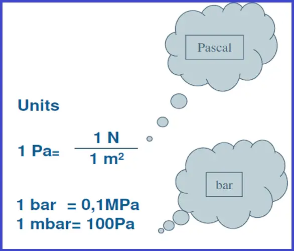
Pressure (P) is defined as Force (F) per Unit Area (A).
Pressure is the action of one force against another force.
The pressure is the force applied to or distributed over a surface.
P = F/A F: Force A: Area
Fig. 1: Units of Pressure
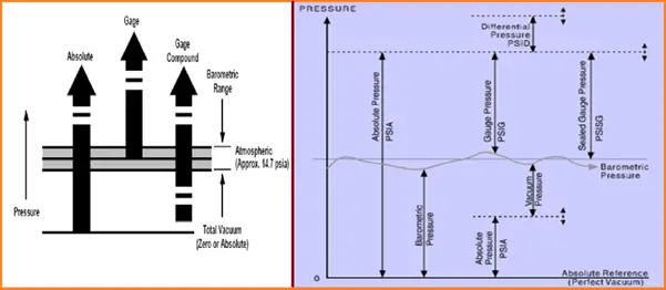
Absolute pressure
Measured above total vacuum or zero absolute.
Zero absolute represents a total lack of pressure.
Range: 0-1 Kg/cm^2 (a)/ 0-1 Bar (a)/ 0-760 mm Hg (a)
Atmospheric pressure: The pressure exerted by the earth’s atmosphere.
Barometric pressure: Same as Atmospheric pressure.
Vacuum Pressure: Pressure below atmospheric.
Fig. 2: Absolute and gage Pressure
Differential pressure: It is the difference in pressure between two points of measurement. In a sense, Absolute Pressure could be considered as a differential pressure with a total vacuum or zero absolute as the reference.
Gauge/Gage pressure: The pressure above the atmosphere is gauge pressure. Represents a positive difference between measured and existing atmospheric pressure. For example – Blood pressure.
Pressure Gauge Formula
The pressure gauge formula is: P = F/A
Where: P = Pressure in Pascals (Pa) F = Force in Newtons (N) A = Area in square meters (m^2)
In this formula, pressure (P) is equal to the force (F) applied per unit area (A). This means that the pressure is directly proportional to the force and inversely proportional to the area.
The pressure gauge formula can be used to calculate the pressure of a fluid or gas by measuring the force applied to a sensing element, such as a Bourdon tube, and dividing it by the area of the sensing element. The resulting pressure can be displayed on a dial or digital readout in units such as pounds per square inch (psi), bar, or kilopascals (kPa), depending on the gauge’s calibration.
Pressure Measurement
The measurement of pressure is considered the basic process variable for measurement of:-
Flow (difference of two pressures).
Level (Head or backpressure).
Temperature (Fluid pressure in a filled thermal system).
The Pressure Measurement System consists of two basic parts:-
A primary element, which is in contact, directly or indirectly, with the pressure medium and interacts with pressure changes.
A secondary element translates this interaction into appropriate values for indicating, recording, and/or controlling.
Common Units of Pressure Measurement
Pressure can be measured using various units depending on the system of measurement and the application. Here are some of the most common units of pressure measurement:
Pascal (Pa):
The SI (International System of Units) unit of pressure.
1 Pascal is equal to 1 Newton per square meter (N/m²).
It is a small unit and is often used for precise scientific measurements.
Kilopascal (kPa):
Equal to 1,000 Pascals.
Commonly used in engineering and everyday applications.
Bar (bar):
Equal to 100,000 Pascals (100 kPa).
Frequently used in Europe for expressing pressure in various contexts.
Atmosphere (atm):
Represents the average atmospheric pressure at sea level on Earth.
Approximately 101.3 kPa or 1.01325 bar.
Millimeters of Mercury (mmHg or Torr):
Originally based on the height of a column of mercury in a barometer.
1 mmHg is approximately 133.322387415 Pa.
Pounds per Square Inch (psi):
Commonly used in the United States and some other countries.
1 psi is approximately 6,894.76 Pa.
Pound-Force per Square Inch (lbf/in²):
Similar to psi but includes the force component.
Used in engineering and aviation.
1 lbf/in² is approximately 6894.76 Pa.
Technical Atmosphere (at):
Equal to 1 kg-force per square centimeter (kgf/cm²).
Used in some industrial contexts, especially in Germany.
Megapascal (MPa):
Equal to 1,000,000 Pascals (1 kPa).
Often used in high-pressure applications.
Newton per Square Millimeter (N/mm²):
Equivalent to 1 Megapascal.
Less common but used in some engineering applications.
Pound per Square Foot (psf):
More commonly used in geotechnical engineering.
1 psf is approximately 47.88 Pa.
Inch of Water (in H2O):
Used for measuring low pressures, such as in HVAC systems.
Typically, 1 in H2O is approximately 248.84 Pa.
Decibar (dbar):
Used primarily in oceanography and marine science.
Equal to 1000 Pascals.
Millibar (mbar):
Equal to 100 Pascals.
Commonly used in weather forecasting.
Dyne per Square Centimeter (dyn/cm²):
A non-SI unit of pressure is often used in older scientific literature.
1 dyn/cm² is equal to 0.1 Pa.
Classification of Pressure Measuring Instruments or Pressure Gauges
Pressure-measuring devices or pressure gauges can be classified on the basis of :
A: Pressure ranges:- Vacuum gage, Draft gage, Low range, compound gage, Medium range, high range, etc.
B: Design principle involved in their operation:
Mechanical movement of the sensing element – e.g. Bourdon gages, Diaphragm gages
Electronic Sensors: e.g. Strain gages, Capacitive, Potentiometric, Resonant wire, Piezoelectric, Magnetic, Optical, etc.
C: On the basis of their application:
Local pressure indication,
Remote pressure indication,
Corrosive service
Pulsating service
Differential pressure measurement
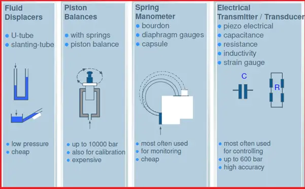
Methods of Pressure Measurement
Fig. 3: Pressure Measurement
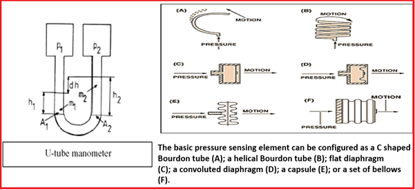
Basic Measurement – U Tube Manometer
A manometer is one of the oldest pressure-measuring instruments and is widely used even in recent times. Their operation is simple and provides accurate results. As the name suggests it is a “U” shaped tube made of glass and partially filled with liquid.
The principle of the manometer is given as P= HEIGHT*DENSITY Where “P” is Pounds /sq. Inch; “HEIGHT” in Inch “ DENSITY” in pounds /Cu. Inch
Advantages of Manometer
Fluids are simple & time-proven
High accuracy & sensitivity
Wide range of filling
Disadvantages of Manometer
No over-range protection
Large & bulky
Measured fluids must be compatible with the manometer fluids
Need for leveling
Fig. 4: U-tube Manometer and sensing element
Pressure Sensing Elements
Pressure Sensing Elements are basically mechanical elements like plates, shells, and tubes. On the application of pressure, these elements deflect which is then converted into physical movement. They are a very important part of pressure-measuring devices.
The main types of sensing elements are Bourdon tubes, diaphragms, capsules, and bellows.
All the above devices, except diaphragms, provide a fairly large displacement. Mechanical gauges use that displacement which is further used by electrical sensors that require significant movement.
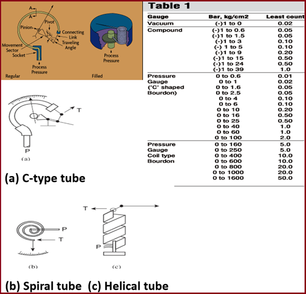
Bourdon Tube Pressure Gauges
The pressure measuring device, the Bourdon tube is the most common. They measure medium to high pressures. The Bourdon tube is basically a curved tube with a circular, coiled, or spiral shape.
It is the twisted tube whose cross-sectional isn’t circular.
Bourdon tube types are c-type, helical type, and spiral type.
They should be filled with oil to limit the damage caused by vibration.
Range: (-)1 to 1600 Kg/cm^2
Advantages of Bourdon Tube
Low cost & simple construction
Wide rangeability
Good accuracy
Adaptable to transducer designs
Disadvantages of Bourdon Tube
Low spring gradient below 50psig
Subject to Hysteresis
Susceptible to shock & vibration
Fig. 5: Bourdon tubes
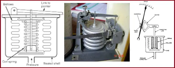
Bellows type Pressure Gauge
Bellows are also used as a pressure measuring instrument. Their main features are
Made of Bronze, S.S., BeCu, Monel, etc..
The movement is proportional to a number of convolutions sensitivity is proportional to size.
In general, a bellows can detect a slightly lower pressure than a diaphragm.
The range is from 0-5 mmHg to 0-2000 psi
Accuracy in the range of 1% span
It is a series of circular parts so formed or joined that they can be expanded axially by pressure. A wide range of springs is employed to limit the travel of bellows.
The measurement is limited from .5 to 70 psi.
It is greatly used as receiving elements for pneumatic recorders, indicators & controllers & also as a differential unit of flow measurement.
Advantages of Bellows Pressure Gauge
High force delivered
Moderate cost
Good in the low to moderate pressure gauge
Disadvantages of Bellows Pressure Gauge
Need ambient temperature pressure compensation
Require spring for accurate characteristics
Limited availability
Fig. 6: Bellows
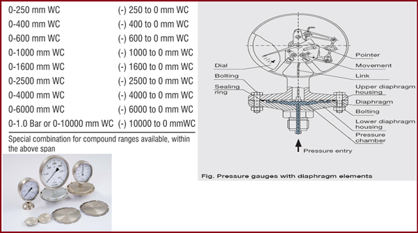
Diaphragm Pressure Gauge
The diaphragm can be used to measure the pressure of both liquids and gases. One circular diaphragm is clamped between a pair of flanges to constitute the pressure-measuring element.
The deflection of a flexible membrane is used for pressure measurement.
For known pressures, the deflection is repeatable. Hence, calibration is possible.
The pressure difference between its two faces dictates the deformation of a thin diaphragm.
The reference face can be opened to the atmosphere to measure gauge pressure, opened to a second port to measure differential pressure, or sealed against a vacuum or other fixed reference pressure to measure absolute pressure. Mechanical, optical, or capacitive techniques are used to measure the deformation. Ceramic and metallic diaphragms are used.
Range: (-) 10000 to (+) 10000 mm-WC
Advantages of Diaphragm pressure gauge
Small size & moderate cost
Linearity
Adaptability to slurry services & absolute & differential pressure.
High over-range characteristics
Disadvantages of Diaphragm pressure gauge
Limited to low pressure
Difficult to repair
Less vibration & shock resistance
Fig. 7: Diaphragm
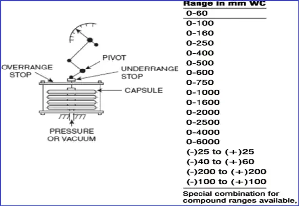
Capsule Pressure Gauge
Capsules as pressure measuring devices are used normally for low-pressure applications.
A capsule is formed by joining the peripheries of two diaphragms through soldering or welding.
Used in some absolute pressure gages.
Fig. 8: Capsules
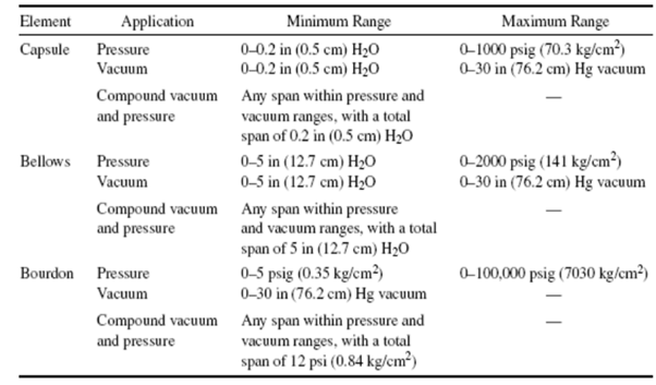
Range of Elastic-Element Pressure Gages
Fig. 9: Range of Elastic-Element Pressure Gages
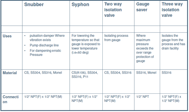
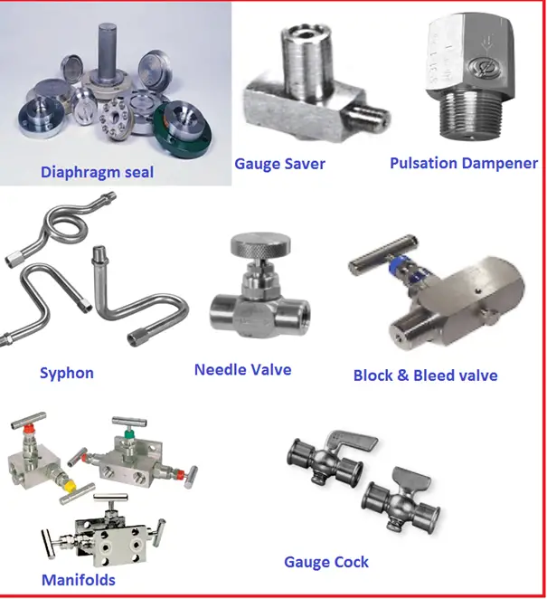
Pressure Measuring Accessories
Fig. 10: Pressure Measuring Accessories
Diaphragm seals: These are designed to isolate the sensing element of pressure gauges from process fluids.
Gauge Saver: Gauge Savers also known as overpressure protectors are applicable where pressures exceed the maximum pressure rating of the pressure gauge.
Pulsation dampener: Dampeners considerably reduce the pulsations and make the gauge reading easier and also improve the life of the gauge.
Siphon: This connection between the pressure gauge & process in applications, where high temperatures like steam, vapors, or fluids are present. It acts as a cooling coil and protects the gauge from high temperatures and also helps in dissipating heat.
Precautions: When first installed the siphon should be filled with water or any other suitable separate liquid.
U Type – For Horizontal pressure tapping
Q Type – For vertical pressure tapping
Needle valve: The large round handle offers maximum ease and precise control to throttle the pressure to the gauge.
Block & Bleed Valve: Equipment Isolation with automatic pressure bleed for safety
Manifolds
These are fluid distribution devices.
These are used in conjunction with pressure gauges, differential pressure gauges & differential pressure transmitters.
They combine instrument isolation & equalizing in one block.
The manifolds are available in 2way, 3 way & 5-way types with remote & direct mounting styles
Gauge cack: It is used in conjunction with the siphon as an isolation valve. It is not recommended for pressure over 100 psi.
Fig. 11: Different Types of Pressure Measuring Instruments
Selection of Pressure Gauges
To ensure accurate measurements and safe operation, the selection of a pressure gauge must be appropriate. However, selecting a pressure gauge is not straightforward as various designs of pressure gauges are available. The selection process depends on various parameters like:
A hazardous area is an area in which an explosive gas atmosphere (flammable gases or vapors, combustible dust, flammable liquids, ignitable fibers, etc.) is present, or maybe expected to be present, in quantities such as to require special precautions for the construction, installation, and use of apparatus. The term hazardous area is associated with the installation of electrical and instrumentation equipment so special design consideration is applied to meet special requirements considering the safety of the operating personnel.
The oil and gas industry involves the handling and processing of flammable and explosive materials, which can create hazardous areas. Some examples of hazardous areas in the oil and gas industry are:
Drilling platforms: Drilling platforms are offshore structures where oil and gas exploration and extraction take place. These platforms have several areas that are classified as hazardous, such as drilling areas, storage areas, and processing equipment.
Refineries: Refineries are facilities that process crude oil into various petroleum products. The processing equipment, storage tanks, and pipelines in refineries are all potentially hazardous areas.
Oil and gas pipelines: Pipelines are used to transport crude oil, natural gas, and petroleum products over long distances. The pipelines and their associated equipment, such as pumps, valves, and compressors, can be classified as hazardous areas.
Gas processing plants: Gas processing plants are facilities that separate natural gas into its component gases and remove impurities. The processing equipment, storage tanks, and pipelines in gas processing plants can all be classified as hazardous areas.
LNG facilities: LNG facilities are used to liquefy natural gas for transportation and storage. The liquefaction process, storage tanks, and associated equipment in LNG facilities are all potentially hazardous areas.
These are just a few examples of hazardous areas in the oil and gas industry. It’s important to identify and classify these areas properly to ensure the safety of personnel and equipment.
What is Hazardous Area Classification?
Hazardous area classification is the scientific evaluation of facilities where the explosive environment is present and classifies them following scientific and engineering principles. To ensure process safety, Hazardous area classification is of utmost importance. Normally, a hazardous area classification is presented on a plan view of plant drawings. These are also known as area classification drawings. To reduce the risk of fire and explosion, the electrical and electronic equipment is installed following the guidelines of hazardous area classification drawings.
During normal operations in chemical and petrochemical facilities, small releases of flammable fluids inevitably happen from time to time. The aim of hazardous area classification is to avoid the ignition of these releases. Area classification focuses on electrical equipment as a potential ignition source in a flammable atmosphere. The approach is to reduce to an acceptable minimum level the probability of coincidence of a flammable atmosphere and an electrical or other source of ignition.
Area classification is the division of a plant or installation into hazardous areas and non-hazardous areas. The hazardous areas are further subdivided into zones.
Purpose of Hazardous Area Classification
Hazardous area classification provides a basis for the selection and protection required for the electrical equipment appropriate to the defined areas. Area classification also helps for the safe positioning of other potential or continuous sources of ignition (eg. fired heaters, Internal combustion engines, gas /turbine drives, plant roads, regulating temporary or portable equipment, etc.). It enables the selection of suitable electrical and instrumentation equipment to ensure a safe work environment.
In recent times, it has been mandatory for chemical plants, oil refineries, LNG plants, sewerage treatment plants, paint manufacturers, distilling, offshore drilling rigs, Spray Booths, Petrochemical complexes, Laboratory and Fume Cupboards to prepare hazardous area classification drawings as hazardous gas vapors are normally present in all such industries.
Please note that it is not the aim of area classification to guard against the ignition of major releases under catastrophic failures of equipment e.g. Rupture of a pressure vessel or a pipeline which has a low probability of occurrence. The risk mitigation for such large releases shall be carried out by proper layout, separation distances, facility sitings, and proper design, maintenance, and operation of the plant.
Hazardous area classification has several advantages in ensuring the safety of personnel and equipment in areas where flammable or explosive materials are present. Some of the advantages are:
Increased safety: Hazardous area classification helps to identify and evaluate the risks associated with the presence of flammable or explosive materials. By identifying the hazards, appropriate safety measures can be implemented to prevent accidents and protect personnel and equipment.
Compliance with regulations: Many countries have regulations and standards that require hazardous area classification in certain industries, such as oil and gas or chemical manufacturing. Compliance with these regulations can help to avoid fines and legal issues.
Cost-effective design: Hazardous area classification can help optimize the design of facilities and equipment by identifying areas that require special protection measures. This can help to reduce costs associated with over-design or unnecessary safety measures.
Effective emergency response: Hazardous area classification helps to ensure that emergency response plans are appropriate for the risks present in the area. This can help to minimize the impact of accidents and improve the effectiveness of response efforts.
Improved communication: Hazardous area classification provides a common language for communication between designers, engineers, and safety professionals. This can help to ensure that all parties have a clear understanding of the hazards and appropriate safety measures.
Overall, hazardous area classification is a critical process in ensuring the safety of personnel and equipment in areas where flammable or explosive materials are present. By properly identifying and evaluating the risks, appropriate safety measures can be implemented to minimize the risk of accidents and protect personnel and equipment.
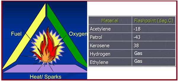
Fire Triangle
Three elements are required to be present together to cause a fire or explosion. These are
Fuel: This is what burns
Oxygen: Required to support fire
Ignition: Heat energy required to start a fire
Refer to Fig. 1 which shows these elements.
Fire/explosion can happen only if all three are present together in an appropriate proposition.
Gas properties
Flashpoint- The lowest liquid temperature at which, under certain standardized conditions, a liquid gives off vapors in a quantity such as to be capable of forming an ignitable vapor/air mixture. It is the vapor that mixes with air to form a flammable vapor.
Fig. 1: Fire Triangle and Flashpoint of a few materials
Lower Explosive Level (LEL): Concentration of flammable gas or vapor in the air, below which the gas atmosphere is not explosive.
Upper Explosive Level (UEL): Concentration of flammable gas or vapor in the air, above which the gas atmosphere is not explosive.
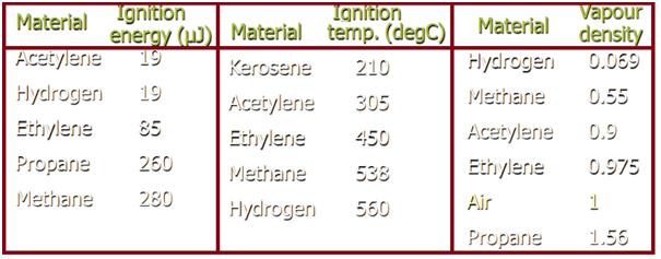
Ignition energy (Fig. 2): Minimum energy of a spark that can ignite a flammable gas or vapor.
Ignition temperature (Fig. 2): The lowest temperature at which flammable gas or vapor gets ignited by itself.
Vapor density (Fig. 2): Density of a vapor or gas relative to the density of air, at the same temperature and pressure.
Fig. 2: Gas properties of various materials
Grades of hazardous release
The release of hazardous elements is grouped as follows:
Continuous grade: Release that is continuous or is expected to occur frequently or for long periods. continuous grade release is present for more than 1000 hours per year (>1000 hours per year). E.g.: Light hydrocarbon interceptor, the seal of a floating roof tank, the area inside a tank, sump, etc.
Primary grade: Release which can be expected to occur periodically or occasionally during normal operation ( > 10 hours per year to < 1000 hours per year). E.g.: Sampling points, equipment nozzle
Secondary grade: Release which is not expected to occur in normal operation and, if it does occur, is likely to do so only infrequently and for short periods (<10 hours per year). E.g.: Piping flanges and valves, instrument fittings, etc.
Such grading is not dependent on the total rate of release or the characteristics of the released material, but only on the probability of the release. Also, some sources may be considered to have a dual grade release with a small continuous or a primary grade and a large secondary grade eg. a vent with a dual purpose or a pump seal.
Steps for Hazardous Area Classification
Following are the general steps for hazardous area classification:
All potential leak sources in the area under review are determined like vents, pump seals, flanges, sample points, instruments, etc.
For each potential leak source the grade of release is determined (that is no. of hours per annum that the leak of flammable material can be expected to occur.
The degree of ventilation in the area around the potential leak source is established (whether there is adequate ventilation or not).
Together it is the grade of release and the degree of ventilation near the potential leak source that determine the type of hazardous zone around the leak source.
The hazard radius around the potential leak source is determined from the category of fluid leaking. The hazard radius forms a horizontal circle around the potential leak and is valid at the elevation of the leak.
From the hazard radius and based on whether the release is lighter or heavier than air and the presence/absence of platforms – the extent of the three-dimensional hazardous zone around the potential leak source is determined.
In a similar way, the hazardous zones from all potential leak sources are determined and superimposed. This gives contours of hazardous areas for the concerned facility both in the horizontal and vertical planes.
Hazardous Area Classification Guide
Two widely used systems are followed in industries for hazardous area classification.
the Class/Division system and
the Zone system
While Canada and the United States predominantly use the class/division system, other parts of the world use the zone system of Hazardous area classification. In the below paragraphs, we will explore the hazardous area zone classification.
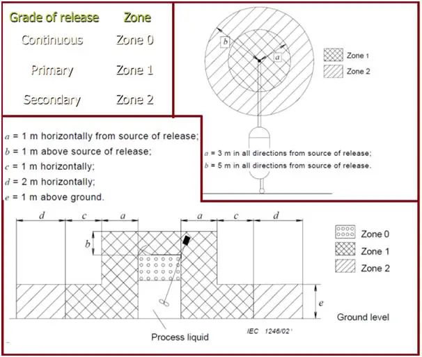
Hazardous Area Zone Classification
The Zone system of hazardous area classification, defines the probability of the hazardous material, gas, or dust, being present in sufficient quantities that can generate explosive or ignitable mixtures. Refer to Fig.3 which shows the hazardous area zone classification based on hazardous gas release grade. There are three zones, Zone 0, Zone 1, and Zone 2.
The grade of release determines the designation of hazardous zones in the immediate vicinity of the release. In open-air situations with adequate ventilation, a secondary grade release will lead to Zone 2, a primary grade release will lead to Zone 1 and a continuous grade release will lead to Zone 0
Fig. 3: Hazardous area zones
Zone classification will be influenced by ventilation also. IEC 60079-10 categorizes ventilation degrees as High, medium, and low. Poor ventilation may push the zone higher by one level. Poor ventilation may result in a more stringent zone while with high ventilation, the converse will be true. A secondary grade source of release may give rise to Zone 1 if local ventilation is restricted. (Example in a sump).
Adequate Ventilation is defined as ventilation sufficient to avoid a flammable atmosphere within a sheltered or enclosed area. This will normally be achieved by a uniform ventilation rate of 12 air changes per hour with no stagnant areas.
Depending on the presence of combustible dust or ignitable fibers and flyings, the hazardous area is classified into three zones: Zone 20, Zone 21, and Zone 22.
In both the above zone classifications, the probability of explosion severity reduces when we move from zone 0 (or zone 20) to zone 2 (zone 22).
The Extent of the Hazardous Area Zone
Distance in any direction from the source of release to the point where the gas/air mixture has been diluted by air to a value below the lower explosive limit. Refer to Fig. 3 above which shows a typical example of a hazardous area zone extent.
Pressure breathing valve (Fig. 3) in the open air, from the process vessel.
A fixed process mixing vessel (Fig. 3); liquids are piped into and out of the vessel through all-welded pipework flanged at the vessel.
For a given release the extent of the zone will vary with the vaporizing potential of the fluid release, the ventilation rate, and the buoyancy of the vapor. The 3rd edition of IP 15 provides three methods for determining the extent of hazardous zones:
Direct Example Approach– limited to common facilities in open areas
Point Source Approach– release rates are dependent on process conditions
Risk-based Approach– an optional rigorous methodology that may reduce the hazardous area determined by the point source approach
The hazard radius for each point of release is a function of fluid characteristics (vapor forming potential) under the circumstances of the release, the release rate, and the rate of vaporization. Hydrocarbon fluids are classified into four fluid categories based on their vaporizing potential.
Fluid Category
Description
A
A flammable liquid that on release would vaporize rapidly and substantially. This category includes: (a)Any LPG or lighter flammable liquid; (b)Any flammable liquid at a temperature sufficient to produce, on release, more than 40% vol. vaporization with no heat input other than from surrounding.
B
A flammable liquid, not in category A, but at a temperature sufficient for boiling to occur on release.
C
A flammable liquid, not in Category A and B, but which can on release be at a temperature above its flash point or form a flammable mist or spray.
D
Flammable gas or vapor (Natural Gas, Hydrogen, etc)
Table: Fluid Category of Petroleum Products
With the fluid category leaking from the particular leak source established, the extent of vapor travel (radii) around the leak source can be determined.
Hazardous Area Classification Drawing
The hazardous area classification drawings are of sufficient scale to show all the main items of equipment and all the buildings in both plan and elevation. The boundaries of all hazardous areas and zones present shall be clearly marked using the clear shading convention for Zone 0, Zone 1, and Zone 2.
It has to be recognized that however, well-protected electrical equipment may be, there will always be a residual risk if it is placed in areas where explosive atmospheres may occur.
Electrical Equipment Selection in Hazardous Area Classification
Once the Hazardous Area classification of a facility is determined, it is used as a basis for selecting suitable electrical equipment. To reach the intended level of safety, equipment must then be installed correctly, operated within its design envelope, and maintained adequately.
As a general policy, electrical equipment should not be located in a hazardous area if it is possible to place it in a non-hazardous area, nor should be placed in Zone 1 if it can be placed in Zone 2. The installation and maintenance requirements for electrical equipment in Zone 1 locations are more stringent than for Zone 2 locations and Zone 0 are more stringent than Zone 1 locations.
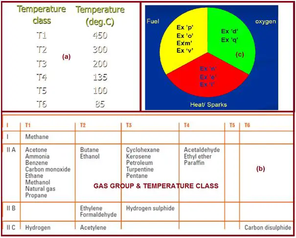
ATEX directives for electrical apparatus for hazardous areas distinguish between two equipment groups as listed below:
Group I – For use in mines (Methane)
Group II – Other than mines
Sub-divisions in group II based on ignition energy requirement
IIA – Atmospheres containing acetone, ammonia, ethyl, alcohol, gasoline, methane, propane, or similar gases
IIB – Atmospheres containing ethylene, acetaldehyde, or similar gases
IIC – Atmospheres containing acetylene, hydrogen, or similar gases
Hazardous Area – Temperature class
Classification based on ignition temperature (Fig. 4 (a)) of gas or vapor. The maximum surface temperature of selected equipment is not to exceed the limiting value.
Fig. 4: Gas group and Temperature Class
Sour area
The area with H2S (Hydrogen Sulphide) concentration above 50 ppm. H2S is highly toxic even in very low concentration
Properties:
LEL – 4% (40,000ppm)
UEL – 46%
Autoignition temperature – 260degC
Gas group IIB
Sour areas with H2S concentration below 4% in the process stream need not be classified as a hazardous area
The Ingress Protection or IP rating
Ingress of moisture or other material could affect electrical equipment and cause it to break down electrically and possibly cause arcs and sparks which could be possible sources of ignition. Also, personnel protection is required against contact with internal live or rotating parts inside the enclosure, and to the apparatus against ingress of solid objects, dust, etc.
The IP rating (or International Protection Rating, sometimes also called Ingress Protection Rating) provides users with more detailed information than vague terms such as waterproof. The IP rating consists of the letters IP followed by two digits.
The first digit indicates the level of protection the fixture provides its internal parts (electrical and moving parts) from the ingress (interaction or contact) of solid foreign objects (like dust). The second digit indicates the protection of the equipment inside the fixture against harmful ingress (contact) with water.
Examples of IP Rating
IP44 is protected against solid objects greater than 1mm (0.04 inches) and liquid sprays from all directions.
IP64 is protected against liquid sprays from all directions.
IP65 is protected against liquid low-pressure jets of water from all directions
IP66 is protected against strong jets of water from all directions
Standards for Hazardous Area Classification
Codes and standards define minimum electrical design and installation requirements for electrical equipment to be used in hazardous areas. The following are some of the codes and standards that are commonly used for hazardous area classification
National Fire Protection Association (NFPA) 70, National Electric Code (NEC): This standard provides guidelines for electrical installations in hazardous locations, including classification of hazardous areas, selection, and installation of electrical equipment, and wiring methods.
American Petroleum Institute (API) RP 500 and RP 505: These standards provide guidance for the classification of hazardous locations in petroleum facilities, including refineries, petrochemical plants, and onshore and offshore production facilities.
International Electrotechnical Commission (IEC) 60079 series: This series of standards provides guidelines for the design, installation, and maintenance of electrical equipment in hazardous areas. The standards cover equipment protection methods, zone classification, and explosion prevention.
Occupational Safety and Health Administration (OSHA) 29 CFR 1910.307: This regulation provides requirements for electrical installations in hazardous locations, including classification of hazardous areas, equipment selection and installation, and wiring methods.
Canadian Standards Association (CSA) C22.1, Canadian Electrical Code: This standard provides requirements for electrical installations in hazardous locations in Canada, including classification of hazardous areas, selection, and installation of electrical equipment, and wiring methods.
IECEx Scheme: This is an international certification scheme for equipment used in explosive atmospheres. The scheme provides a framework for conformity assessment of equipment and systems, including testing, certification, and ongoing surveillance.
IP 15
DEP 80.00.10.10
ATEX – EU Directives
The hazardous area classification and location of equipment must be ascertained before the choice of appropriately certified electrical equipment is made.
Hazardous Area Classification FAQs
What is a hazardous area classification chart?
A hazardous area classification chart is a graphical representation of the classification of hazardous areas according to the types of hazardous materials present and their potential for ignition. The chart typically includes a legend that describes the various types of hazardous materials and the criteria used to classify them.
The hazardous area classification chart is used to identify and evaluate the risks associated with the presence of flammable or explosive materials in a particular area. The chart provides a visual reference for the classification of the area and the associated safety measures that must be implemented.
The chart typically includes several zones, which are defined by the probability of the presence of flammable materials and the duration of their presence. The zones are used to determine the type of equipment and safety measures that must be used in each area. For example, Zone 0 is an area where flammable materials are present continuously or for long periods of time, while Zone 2 is an area where flammable materials are present only intermittently or in small quantities.
The hazardous area classification chart is an important tool in the design, construction, and maintenance of facilities where flammable or explosive materials are present. It helps to ensure that appropriate safety measures are implemented to protect personnel and equipment from potential hazards.
What are the differences between NEC hazardous area classification and NFPA hazardous area classification?
The NEC (National Electric Code) and NFPA (National Fire Protection Association) are two organizations that provide guidelines for hazardous area classification. While there are some similarities between their guidelines, there are also some differences.
One key difference between the NEC and NFPA guidelines is their approach to classification. The NEC provides specific requirements for classifying hazardous locations based on the types of materials present, while the NFPA provides general guidelines for assessing the potential for ignition based on factors such as temperature, pressure, and ventilation.
Another difference is in the terminology used for hazardous area classification. The NEC uses Class, Division, and Group to describe hazardous areas, while the NFPA uses Class and Division. The definitions of these terms can also differ slightly between the two organizations.
In terms of the industries they serve, the NEC is primarily focused on electrical installations and equipment, while the NFPA covers a wider range of fire protection and safety issues.
Despite these differences, both the NEC and NFPA guidelines are widely recognized and used in hazardous area classification. It’s important to understand the specific requirements and terminology used by each organization when applying their guidelines to a particular situation.
What are the three classes of hazardous locations?
The three classes of hazardous locations are defined by the National Electric Code (NEC) in the United States. They are:
Class I: Locations where flammable gases or vapors are present in the air in sufficient quantities to produce explosive or ignitable mixtures. Class I locations are further divided into Division 1 and Division 2, depending on the likelihood and duration of the presence of these materials.
Class II: Locations where combustible dust is present in sufficient quantities to produce explosive or ignitable mixtures. Class II locations are also divided into Division 1 and Division 2.
Class III: Locations where easily ignitable fibers or materials producing combustible flyings are handled, stored, or processed. Class III locations are not divided into divisions.
The classification of a hazardous location is important for determining the appropriate electrical equipment and wiring methods that can be used in that location. This helps to reduce the risk of ignition and explosion caused by electrical equipment.
References and Further Reading for Hazardous Area Classification Guide
In piping stress analysis, both the subject terms i.e, Sustained Stress and Expansion Stress are widely used. For all the piping systems which need analysis, the calculated sustained and expansion stresses have to be kept below code allowable stress. In the following tutorial, both of these stresses are clearly explained.
What is Sustained Stress?
Sustained stress is one of the primary stress caused by primary loads’ Weight (Pipe Weight, Insulation Weight, Fluid weight, etc) and Pressure (Internal and External Pressure). This stress is present in the piping system throughout the plant operating life. This means this stress will remain as long as the piping system survives and that’s why it is very important to calculate the piping sustained stresses and keep the stresses below code allowable values.
ASME B31 codes provide equations for sustained stress calculation and also provide allowable values to compare the calculated stress. The allowable stress value and equation for the calculation of sustained stress vary from one piping code to another.
What is Expansion Stress?
Expansion stress is displacement-driven secondary stress generated in the piping system due to temperature change or thermal differential from the installed to operating temperature.
Whenever the temperature of a piping system changes from one value to another, the system starts to move (expansion or contraction). If this free thermal movement is restricted then thermal stresses will be generated in the system.
It is obvious that Piping systems in process or power industries are connected to some equipment or other piping. This means free thermal movement is restricted which causes to increase the thermal stress.
All B31 codes provide an equation for calculating this expansion stress and then compare the calculated stress with allowable values.
A Typical Stress System in Caesar II
Basics of Sustained and expansion Stress in Piping System
The following two video tutorials nicely explain the basics of sustained and expansion stress in a piping system
Video Tutorial 1:
Video tutorial-1: Sustained and Expansion Stress in Piping System
Video Tutorial-2:
Video tutorial-2: Sustained and Expansion Stress in Piping System
Composites are novel materials made by combining two or more materials, the resultants of which possess the combination of better properties of the ingredients.
Constituents of composites
Base material – Matrix – metal, ceramic, or polymer
Reinforcement – e.g. fiber
Fillers
Dual Laminate Composite
Thermoplastics lined to thermosets e.g. PVC-FRP, CPVC-FRP, PVDF-FRP, ECTFE-FRP, PP-FRP, FRP-FRP
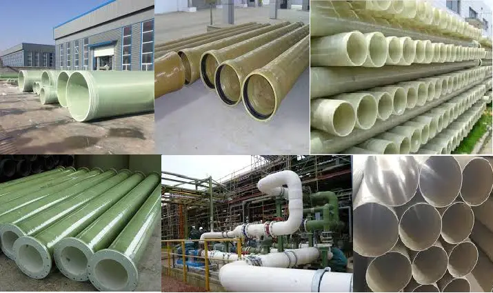
FRP – made of fiberglass impregnated with either –
Unsaturated polyester resin
Vinyl ester resin
Furan resin
Fiberglass – provides structural stability
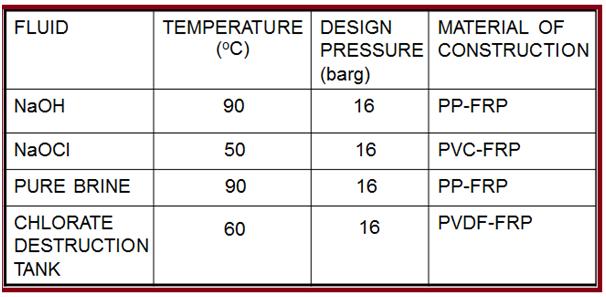
Fig. 1: Service conditions for dual laminate composites
Carbon fibers – superior mechanical properties, low density, and corrosion resistance used for offshore oil field applications
For some strength: CFRP composite
80% lighter than steel
60% lighter than aluminum
Applications of GRP composites
Resistant to most chemicals including acids, where metals like SS and Ni-alloys fail to survive Also handle lethal and corrosive Chlorine gas, halide salts, and bleaching solutions including hypochlorite Unlike metals can withstand wide fluctuations in pH and temperature. E.g. effluent treatment process Resistant to corrosion in damp soil conditions, oxidizing and reducing agents such as H2S
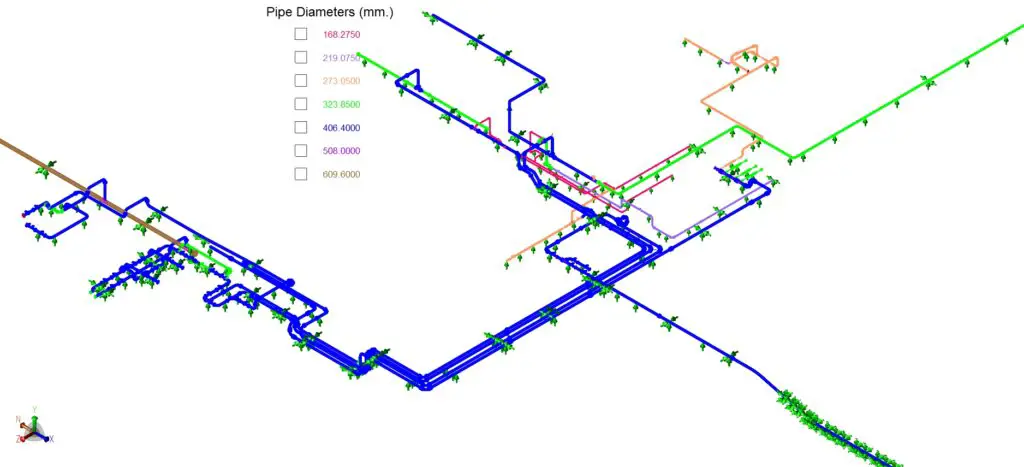
High-pressure pipelines handling aggressive media such as saltwater, oil, or brine
Unsaturated polyester, vinyl ester resin used for chimneys and Stacks.
Can withstand high temperatures (up to 240 Degrees C) and severe corrosive gases
Carbon fiber reinforcements and epoxy resins are used only in selective cases, wherein high strength and light weight are more important than corrosion resistance.
Deep well platforms – tension leg platforms(TLPs)
spars and drilling risers
choke and kill lines
Offshore Applications
Secondary structures including ladders, handrails, and gratings
Flow and gathering lines
Firewater lines
Casings
Surface injection
Saltwater disposal lines
CO2 handling
Tank battery piping
Materials used in Offshore composites
Bisphenol(A) polyester, bisphenol vinyl ester, Novalac epoxy, and phenolics – Fire retardant
Summary
Glass fiber-reinforced composites are being selectively used in chemical processes and oil & gas industries for the following advantages:
Exceptional freedom of design and manufacture of many complex shapes.
Outstanding durability even in extremely harsh environments
A custom selection of resin and reinforcements
Superior strength and stiffness-to-weight ratios
Highly corrosion resistant in almost every chemical environment
Lower maintenance and replacement costs
Glass Lining
Glass
Inert, hard, and biologically inactive
Can be formed into a very smooth and impervious surface
Brittle in nature
Types of Pfaudler Glass
World Wide Glasteel 9100
Pharma Glass PPG
Stainless Steel Glass 4000
Ultra Glass-6500
Anti-static Glass
World Wide Glasteel 9100
Offers an unmatched combination of
Corrosion resistance
Impact Strength
Thermal shock resistance
Non-adherence
Heat transfer efficiency
Stainless Steel Glass 4000
Reliable glass lining of stainless steel for pharmaceutical / FDA applications
Suitable for cryogenic processes & pure products for electronics
A virtually inert glass that resists corrosion, abrasion, and product adherence
Pfaudler Ultra Glass
Addresses the requirement of chemical reactions at high temperatures
Enhanced thermal tolerance up to 343 Degrees C – an improvement over WWG 9100
Extended thermal shock protection for faster heating and cooling
Limitations:
Operating temperature
Chemicals
Cavitation
Electrostatic discharge
Abrasion
FRP
What is FRP?
FRP is a resin lining into which layers of Fibers are incorporated to optimize lining structure capability and performance.
FRP is widely used because of its relatively low cost, good chemical resistance, and its mechanical properties:
Specific tensile strength (GPacm3/gm) – Tensile strength per unit density
Specific stiffness (GPacm3/gm) – Tensile modulus per unit density
Scope of Use of FRP
The bottom lining of AST
Piping
Automotive
Naval
Aerospace
Why tank lining?
An effective method for preventing internal corrosion in storage tanks
Maintaining the stored chemicals’ purity and quality
The long lifetime for storage tanks
To overcome tank bottom perforations due to external corrosion
Graphite
Impervious Graphite is a traditional material selected for high conductivity, chemical resistance, and good mechanical properties. It is specially treated with synthetic resins to ensure that the base structure is fully impervious to liquids under pressure.
Graphite forms no compounds due to corrosion, and no surface films as do many metals. Hence graphite surface remains smooth and more resistant to scale build-up.
Graphite lining can replace most of the other types of linings due to:
Better thermal conductivity
Superior chemical corrosion resistance. Corrosion loss is < 0.05mm/yr
Lower initial/lifetime costs
Has higher temperature applications compared to all the polymeric linings except for the PTFE family