What is Fluid Flow?

Written by Anup Kumar Dey in Process

Fluid Flow is generally measured inferentially by measuring velocity through a known area. With this indirect method, the flow measurement is the volume flow rate ”Q” stated in its simplest terms.

Volume flow rate (Q)

It is expressed as a volume delivered per unit time and typical units are gallons/min, m³/hr, and ft³/hr.
Q = A * V

Where: A is the cross-sectional area of the pipe & V is the fluid velocity.

Mass or weight flow rate

Expressed as mass or weight flowing per unit time. Typical units are kg/hr, Ib/hr.

This is related to the volume flow rate by F = p * Q

where

F = Mass or Weight flow rate.
p = mass density or weight density.
Q = volume flow rate

Factors affecting Flow in Pipes

Velocity (V) of the fluid.
The friction of the fluid in contact with the pipe.
Viscosity (µ) of the fluid.
The density of the fluid.

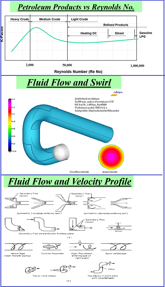
The most important flow factors can be correlated together into a dimensionless parameter called the Reynolds number. It describes the flow for all velocities, viscosities, and pipeline sizes.

In general, it defines the ratio of velocity forces driving the fluid to the viscous forces restraining the fluid, or:

R_D = VDρ/µ

D=Diameter ;

Fluid Flow in Pipes

At very low velocities or high viscosities, R_D (Reynolds Number) is low and the fluid flows in smooth layers with the highest velocity at the center of the pipe and low velocities at the pipe wall where the viscous forces restrain it. This type of flow is called laminar flow and is represented by Reynolds numbers below 2,000. One significant characteristic of laminar flow is the parabolic shape of its velocity profile

At higher velocities or low viscosities, the flow breaks up into turbulent eddies where the majority of flow through the pipe has the same average velocity. In the “turbulent” flow the fluid viscosity is less significant and the velocity profile takes on a much more uniform shape.

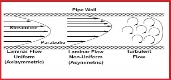
Turbulent flow is represented by Reynolds numbers above 4,000. Between Reynolds number values of 2,000 and 4,000, the flow is said to be in transition.

Measurement of Fluid Flow inside a Pipe

The type of device used often depends on the nature of the fluid and the process conditions under which it is measured.

Flow is usually measured indirectly by first measuring a differential pressure or a fluid velocity. This measurement is then related to the volume rate electronically.

Flow meters can be grouped into the following generic types:

Head Type Flow Meters– Orifice Plates, Venturi, Flow Nozzles, Pitot Tubes, etc.
Target Flow Meters.
Positive Displacement Type Flow Meters such as Nutating Disc, Rotating Valve, Oval Gear, Oscillating Piston, Roots (Rotating Lobes), Rotating Impeller, etc.
Velocity Type Flow Meters such as Turbine Meters, Electromagnetic Flow Meters, Vortex Flow Meters, Ultrasonic Flow Meters, etc.
Mass Flow Meters such as Thermal Mass Flow Meters, Coriolis Mass Flow Meters, etc

All the above flow meter types will be explained in my future articles.

Flow Fundamentals

Accurate Measurement Requires the Right Meter Choice for the Application

Newtonian fluid

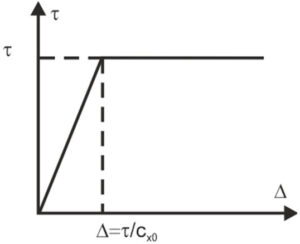
A Newtonian fluid is defined as a fluid that, when acted upon by applied shearing stress, has a velocity gradient that is solely proportional to the applied stress. Petroleum products and most mixtures of particles in petroleum products are Newtonian fluids.

The accuracy of flow meters is based on the steady flow of a homogenous, single-phase Newtonian fluid, and for turbine and ultrasonic meters a defined velocity profile does not alter the coefficient in long, straight runs of pipe.

Raynolds Number

A dimensionless parameter expressing the ratio between the inertia (driving) and viscous (retarding) forces.

It is given by the formulas:

Re = 2214 x BPH / (D x n)

Re = 351 x M³/hr / (D x n)

where: The flow rate is in BPH barrels/hour (or M3/hr); D is the diameter of the meter in inches and n is the kinematic viscosity of the fluid.

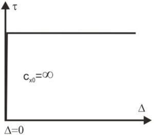
Fig. 2 below shows the curves for flow profile vs Reynolds number and Flow profile vs Performance

Fig. 2: Flow profile

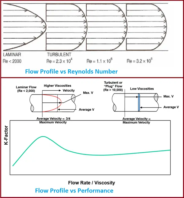
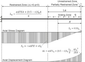
Figure 3 shows various curves/profiles related to Fluid Flow.

**Fig. 3: Fluid flow and velocity profiles.**

What is Restrained and Unrestrained Pipes: Part 2

Written by Alex Matveev in Caesar II,Piping Stress Analysis,Piping Stress Basics,Start-Prof

Start-Prof is a part of PASS software suite for piping stress analysis, hydraulics analysis, boiler & pressure vessel, heat exchanger, column, tank design & stress analysis is available worldwide since 2018.

Continued from Part 1

Restrained and Unrestrained Zones in the Buried Pipelines

Buried gas and oil pipelines usually are very long and have a small temperature difference. In this case all three types of pipe condition occur: unrestrained, totally restrained and partially restrained.

Let’s assume that soil model is ideal plastic:

In this case the axial stress and axial displacement diagram along the pipeline will be as follows:

Unrestrained, Partially Restrained, and Unrestrained Zones in Buried Pipeline with an Anchor on the Left End and Free Right End With Ideal Plastic Soil Model

As we see unrestrained zone on the right end of the pipe is a very small. The most length of pipeline consists of totally restrained and partially restrained zones.

Anchor load in restrained zone will be:

Axial force at restrained zone is:

Stress at restrained zone is:

Axial force at unrestrained zone is:

Stress at unrestrained zone is:

Balance equation:

Therefore virtual anchor length is

Stress function in unrestrained zone is:

Displacement function in unrestrained zone is:

Axial displacement at restrained zone should be zero. Therefore:

Axial displacement at the right end of the pipe will be

For more complex and more realistic Elastic-plastic soil model that is used in PASS/Start-Prof pipe stress analysis software the zero displacement (totally restrained) zones is absent:

Let’s assume that restrained zone begins when axial displacement is very small, for example 1% of maximum displacement. Bypassing complex calculations the sliding zone length that is used in PASS/Start-Prof software is:

Virtual anchor length using FEM procedure can be calculated in PASS/Start-Prof Software using Start-Elements module:

Start-Elements Procedure for Virtial Anchor Length Calculation

Strength Criteria in ASME B31.4 and B31.8 Codes

In real design practice the determination of the restrained zones is very time consuming. For example on the screenshot below the restrained zones of a very long gas pipeline are shown.

That’s why we decided to create universal strength criteria that automatically meets the B31.4 and B31.8 code strength requirements, but can be used for any type of piping. The problem is that ASME B31.4-2016 and B31.8-2016 has unclear requirements for stress analysis.

ASME B31.4 code, paragraph 402.6.2 requires longitudinal stress in unrestrained pipe to be less than 0.75Sy for sustained loads and 0.8Sy for occasional loads.

This requirement can be extended for all pipe conditions, no matter restrained or unrestrained, but for primary loads. Longitudinal stress in any type of piping from sustained primary loads (weight and pressure) should be less than 0.75Sy:

M and Fa should be calculated by software including Bourdon effect.

ASME B31.4 code, paragraph 402.6.1 requires longitudinal stress in restrained pipes to be less than 0.9Sy, the equivalent stress should be less than 0.9Sy

This requirement can also be extended for all pipe conditions, but for primary and secondary loads acting simultaneously (weight, pressure, and thermal expansion).

M and Fa should also be calculated by software including Bourdon effect. In this case axial pressure stress will be correct for both restrained and unrestrained zones.

The expansion stress should be checked for both restrained and unrestrained pipes.

The same way ASME B31.8 strength criteria can be improved.

The summary of suggested strength criteria for ASME B31.4 and B31.8 shown in the following tables.

Table 1. Original ASME B31.4-2016 Strength Criteria

Start Smart Check ASME B31.4-2016 Improved Strength Criteria

Table 3. Original ASME B31.8-2016 Strength Criteria

Table 4. Start Smart Check ASME B31.8-2016 Improved Strength Criteria

We already implemented the improved ASME B31.4 and B31.8 strength criteria into PASS/Start-Prof software and call it “Start Smart Check”. Every user can select this option and forget about manual selection of restrained and unrestrained pipes in stress analysis software.

Selection of Start Smart Check Option in PASS/Start-Prof

Also we added “manual” and “Autodetect” options. Using “manual” option user should select restrained or unrestrained option for each pipe. If “Autodetect” option is selected, Start-Prof automatically use equations for restrained pipe if following condition is truth:

Manual option is not recommended because it seriously slows down the design process. Autodetect option is not recommended because the strength criteria will be sometimes too conservative and sometimes less conservative for partially restrained pipes.

We recommend users to select “Start Smart Check” option by default because the similar criteria are already used successfully in Start-Prof (GOST codes) for buried pipelines for many years and proved their reliability. You can just draw pipeline and run analysis. There’s no need to divide it into restrained and unrestrained.

Related video about buried piping analysis:

More than 100 Chinese companies choose START-PROF for buried district heating networks analysis with CJJ/T 81-2013 code is used instead of ASME B31.4. CJJ/T 81-2013 is adopted version of GOST 55596-2013 code. This code is free from described above problems, and ideas of ASME B31.4 and B31.8 code improvment in this article was taken from GOST 55596-2013 code.

Example: District heating buried piping network in Universal Studios Park in Beijing calculated using PASS/START-PROF

Pipeline Stress Analysis

Written by Anup Kumar Dey in Caesar II,Pipeline,Piping Stress Analysis,Piping Stress Basics

Pipeline Stress Analysis is quite different from normal plant piping stress analysis. Normally Pipelines run kilometers in length for transferring oil, gas, water, or sewer. There are two types of pipelines. Liquid Pipelines and Gas pipelines. Pipeline Stress Analysis of liquids is governed by ASME B31.4 whereas the same design standard for gas pipelines is dictated by ASME B31.8.

All my previous articles on this website describe the stress analysis methodology of piping systems using Caesar II based on ASME B31.3. But I received requests from many pipeline engineers to describe the pipeline stress analysis methodology. So in this article, we will explore the required steps for stress analysis of a pipeline system.

Pipeline Stress Analysis Considerations

The most fundamental difference between pipeline and plant piping is the very long length of the pipeline. A pipeline with kilometers in length produces a very large amount of expansion even though the design temperature of pipelines is normally less as compared to plant piping. A reasonable estimate of the movement and its interaction with the end resistance force afforded by connecting piping and equipment are very important aspects of designing a pipeline.

Pipeline thicknesses are generally less than plant piping thicknesses. It’s quite obvious to reduce pipeline material costs. Also, normally API 5L material is used.

Pipeline General Arrangement Drawings are used for showing pipeline routes. These pipelines in most cases do not run parallel to any given direction. Refer to Fig. 1 for a typical sample of pipeline GA/Route plan drawing.

**Fig. 1: Sample GA for pipeline Stress Analysis**

A large amount of pipeline movements are caused due to pressure elongation, also known as the bourdon effect. For plant piping bourdon effect is normally ignored but for pipelines, the pressure elongation is significant and is considered. So,

The total elongation for pipelines=Temperature Elongation+Pressure Elongation.

Pipeline stress Analysis is not as stringent as plant piping as the allowable values are much more as compared to plant piping allowable values.

Hydro-test pressure for pipeline stress analysis is normally considered as 1.25 times the design pressure which is less than the plant piping design pressure consideration.

The pipeline may be above-ground with road and wadi crossings or completely buried.

Pipeline Stress Analysis Software

Pipeline stress analysis software is the same as plant piping stress analysis software as all those software have the provision for changing the design code and running the analysis. So all the below-mentioned software are used as popular pipeline stress analysis software

Caesar II by Hexagon
Auto-Pipe by Bentley
Start-Prof by PASS
Caepipe
Rohr II

Pipeline Stress Analysis Calculations

Pipeline Stress Analysis is performed for Sustained, Operating, Occasional, and Expansion Load Cases. The load cases are similar to plant piping analysis load cases. The main features for pipeline modeling are listed below:

Pipelines possess a very long radius (25 D to 60 D) elbows. So bend radius must be provided.
The buried depth of cover must be accurately entered into the soil parameters. Different pipeline segments normally have different buried depths as pipelines normally run on uneven surfaces.
If pipe sleeves are used in buried parts those have to be modeled as above-ground parts with spacer supports at even distances.
Normally expansion loops are provided at a distance of 500 m from the other expansion loop for above-ground pipelines.
Pipelines turn at various angles (not 45 degrees or 90 degrees similar to plant piping) so those need to be modeled correctly from pipeline GA drawing.
Pipeline models are created from Pipeline General Arrangement drawings or Route Plan Drawings (Refer to Fig 1 for a sample). Isometrics are not available similar to plant piping.
In most cases, the aboveground and buried pipeline design temperature is different and needs to enter correctly.
For buried parts of pipelines, proper soil data must be entered from soil reports by the civil team.
There are no S_h values similar to B31.3. A pipeline normally runs for several kilometers without any fittings attached. Because of such simplicity, the stress in the majority portion of a pipeline is quite predictable. Taking advantage of this characteristic, the code’s allowable stress for a pipeline is greatly increased, as compared to that for plant piping. All allowable values are linked with S_y (Specified Minimum Yield Strength) as the allowable stress of a pipeline is mainly to protect the pipe from gross deformation. Whenever you select B31.4 or B31.8 in Caesar II all S_h value fields become grey.
There is nothing like liberal stress in pipeline stress analysis.
Pipelines are always connected with piping systems. So in the same stress system, both piping and pipeline codes may be required to use.

The following figure shows a typical pipeline as modeled using pipeline stress analysis software Caesar II

**Fig. 2: Pipeline Stress System in Caesar II**

Pipeline Stress Analysis Basics

The basic equations for pipeline stress analysis are provided by the following codes and vary from one code to another. So readers are requested to refer to the following codes and standards for a better understanding of pipeline stress analysis basics.

ASME B31.4 for liquid and slurry pipeline stress analysis
ASME B31.8 for gas pipeline stress analysis
ISO 14692 for pipelines made of GRE/GRP/FRP materials
AWWA M 45 for big-size water pipelines.

Online Video Courses related to Pipeline Engineering

If you wish to explore more about pipeline engineering, you can opt for the following video courses

Process Design of Centrifugal Compressor System

Written by Anup Kumar Dey in Mechanical,Piping Interface,Process

Process Datasheet

Defines the suction and discharge conditions (Pressure, Temperature, Flowrate) and gas composition.
The main input to the compressor vendor.
Define all possible options of suction and discharge conditions and gas compositions, present, and future.
The vendor selects the model which fits these conditions the best.

Compressor performance curves

Input from the compressor vendor
Relationship of Flow vs. Head (polytropic, isentropic)
Surge point and choking (stone wall)
Variation with RPM
Input to HYSYS for the generation of performance at different conditions

Performance data

Input from compressor vendor.
Defines the interstage pressures and temperatures.
Gives input for the HYSYS simulation.

Process Simulation

HYSYS simulation model
Based on the Compressor performance data
Forms the basis for material and energy balance.
Defines the cooler heat duty.
Generates property data for the calculations.

System components

Compressor and Motor
Coupling (e.g. Voith)
Lube oil System
Seal oil / Seal gas system
Scrubbers
Piping and Instrumentation
Air Coolers

Advantages Seal gas system

No seal oil system required
No need to dispose of/clean up contaminated oil
Eliminates fouling problems due to oil ingress in process streams
Less gas loss
The dry gas seal advantages significantly outweigh the seal oil benefits

Process Calculations

Settle out Calculations
Blowdown calculation
Pipe sizing calculations
Hydrate calculations

Settle out calculation

Equalized pressure during a compressor shutdown.
High-pressure trip conditions are taken as pressures before settling out.
Enthalpy balance of the system.
It can be done using a spreadsheet or HYSYS.
It can define the design pressure for some of the sections.

Blowdown calculation

Intent: Reduce the pressure of the equipment to 50% of the design pressure within 15 minutes during a fire emergency.
Typically done using Dynamic depressurizing Utility in HYSYS
Relief valves are not depressurization devices.
Ball valve + Orifice combination OR control valve

The blowdown calculation takes the following into account:

Vaporization of liquid due to pressure reduction,
Vaporization due to heat input from the external fire,
Pressure after 15 minutes is reduced from design pressure to 50% of design pressure,
Start at settle-out conditions.
The gas compressor system is blocked in and no additional mass is fed into the system during blowdown.
Maximum allowable depressurization rate for the compressor O-rings of 20 bar/min,
There is no other heat input into the system other than fire.
The relief rate calculated is not limited by the flare.
Use to find the lowest temperature attained and hydrate formation possibilities.
Uncontrolled vs. Staged Blowdown

**Fig. 3: Uncontrolled vs. Staged Blowdown**

Pipe sizing calculations

Importance of pressure drop and machine performance.
Tools used.
Cooler header sizing.
Avoiding loops in suction.
Provision of drain boots.

Hydrate calculations

Hydrates are ice-like non-stoichiometric crystal structures composed of water molecules engaging natural gas molecules.
The solid formation chokes piping.
Flow problems.
The formation depends on P, and T conditions and composition.
Predicted by HYSYS.

Gas Blow-by calculations

Caused by losing liquid level in the scrubbers.
High-pressure gas flows into the low-pressure system potentially overpressurizing it.
Calculations are done to ensure that the downstream system is adequately protected.
The control valve is considered to be fully open during this case.
The highest operating pressure of the upstream system is considered for sizing.

Scrubbers

Vertical Knock out vessels.
Limit liquid carries over to the compressors.
Internals – SMS / SV / SVS

Air Coolers

Heat duty based on Process Simulation.
Process parameters based on the simulation.
The vendor does the sizing with HTRI or other proprietary software.
Pressure drop is critical.

Flare and Blowdown system

The flare system needs to be designed for
Blowdown depressurizing load.
Flaring due to compressor trip
Fire case relief
Blocked discharge of the compressor
The flare system may require a KOD based on the quality of the gas flared. (Liquid presence)

Control Philosophy

Capacity control
Antisurge control
Scrubber level control

Safeguarding philosophy

Process shutdown.
Emergency shutdown.
Other shutdowns.

Process shutdown

Close the discharge ESD valve. The suction ESD valve shall remain in an open position. The blowdown ESD valve shall remain in a closed position. The antisurge valves and capacity control valve goes to the open position. The motor stops and the compressor settles out to suction pressure. The auxiliaries keep running.
Generally initiated on trips on process parameters.
Enables faster start-up compared to ESD

Emergency shutdown

PSD1 shall Trip the compressor motor & auxiliaries, and Close the ESD valve on the suction and discharge header.
The antisurge valves and capacity control valve goes to the open position.
The external seal gas supply shall be isolated by the ESD valve on the seal gas line.
The compressor blowdown valves shall open and depressurize the gas to flare.
Initiated on Fire, Station ESD.

Other shutdowns

The suction, inter-stage(s), and discharge scrubbers low-level close liquid outlet ESD valves.
The inter-stage(s) and After-cooler fan high vibration shall trip the respective fan.
Low temperature at the aftercooler outlet shall trip the first working fan at 30 deg C and the next at 20 deg C.
External seal gas high pressure downstream of external seal gas pressure letdown valve for LP casing shall close the external seal gas supply ESD valve.

Few more useful resources for you…

Articles related to Compressor
Articles Related to Pumps
Piping Design and Layout Basics
Piping Stress Analysis Basics
Piping Materials Basics
Articles Related to Mechanical Design
Articles Related to Process Design
Articles Related to Heat Exchanger

Material Selection & Quality Management for a Cross Country Pipeline

Written by Anup Kumar Dey in Engineering Materials,Pipeline,Piping Design Basics,Piping Interface

Cross Country Pipelines are very long-distance pipelines that run outside of the battery limit of the processing plants. The design of cross-country pipelines is governed by ASME B31.8 or ASME B31.4 for gas and liquid pipelines respectively. The pipeline material selection is a very important activity. The material selection of cross-country pipelines needs the overall knowledge of:

Design considerations.
Construction ease considerations.
operations and maintenance considerations.
hazards, risks, safety considerations and
overall economic considerations

Various codes and standards list the mandatory requirements during pipeline material selection but the final selection is optimized with user experience. The following paragraphs will list some important considerations for cross-country pipeline material selection.

Typical cross country Pipeline — **Fig. 1: Typical cross-country Pipeline**

Pipeline Material Selection Considerations

The following points need to be addressed while selecting cross-country pipeline materials

Line pipe material
Soil material
Backfill material
Sacrificial anodes
Pipeline Component materials
Coating & Insulation
The physical and mechanical properties of the material.
Resistance to corrosion.
Ability to cut, machine, bend and perform other fabricating operations.
The life span of material.
Cost of material.
Ability to withstand hazards during pipeline construction and service.

Cross Country Pipeline materials

Normally, the following pipe materials are used as cross-country pipeline materials.

Copper alloys, particularly the copper-nickel series
Bare carbon steel
Galvanized steel
Carbon steel internally coated or lined (e.g. with paint, bitumen, rubber, cement)
Stainless steels
Plastics or reinforced plastics
Titanium.

Composition of steel pipeline

A typical, modern line pipe steel will have

carbon — 0.10 to 0.15%,
Manganese — 0.80 to 1.60%,
Silicon — 0.40%
Phosphorus below 0.020%
Sulfur below 0.010%,
less than 0.5% -copper, nickel, and chromium.

Development of plain carbon steel pipes to the high-end TMCP steel pipes:

Improved strength, both yield, and ultimate tensile strength
Improved toughness properties, i.e. the lowering of transition temperature from brittle to ductile fracture and an increase of the impact toughness.
Improved weldability.
Improved resistance towards hydrogen-related disintegration in sour service, i.e. due to exposure to a wet H2S-containing environment.

Increase of yield strength and ultimate tensile strength by alloying:

**Fig. 2: Alloying Elements for Pipeline Materials**

Soil materials

It is primarily strength and friction properties that are a concern in pipe-soil interaction.
Classification of soil is based on a visual inspection and laboratory testing.
The aim of the investigation is to classify the soil so that strength parameters can be determined.

Cohesive soil consistency classification

Non-cohesive soil characterization

**Fig. 4: Non-Cohesive Soil Characteristics**

ASTM D422-63 Standard test method for particle-size analysis of soils:

ρ_r = (e_max − e)/(e_max − e_min)

where

e_max void ratio of the soil in its loosest state
e in situ void ratio
e_min void ratio of the soil in its densest state.

Backfilling Material

Fertility of Agriculture fields

Sacrificial anodes

Sacrificial anodes are used for cathodic protection of the line pipe steel.
the traditional sacrificial anode materials for application are alloys based on zinc or aluminum, although other metals may be used (such as carbon steel to protect stainless steel line pipe).
Electrochemically the anode materials are characterized by the current capacity (measured in Ah/kg) and the closed-circuit potential (measured in V). Density (kg/m3) is the only relevant physical parameter.

Composition of zinc anode alloy

Composition of aluminum anode alloy

**Fig. 6: Composition of Aluminium Anode Alloy**

Pipeline component materials

The pipeline system components other than the line pipe material itself are:

valves;
isolation couplings;
flanges;
branch connections (tees, wyes, o-lets, etc.);
reinforcement sleeves (e.g. crack arrestors, buckle arrestors);
brackets and support structures at valve stations and pipeline crossings.

ASME B31.4 Standards

Pipe, Steel, Black & Hot-Dipped, Zinc-Coated Welded& Seamless —- ASTM A53.
Seamless Carbon Steel Pipe for High Temperature —- ASTM A106.
Pipe Flanges & Flanged Fittings —- ASME B16.5.
Steel Valves, Flanged & Butt-welding End —- ASME B16.34.
Steel Pipe Flanges —- MSS SP-44.
Steel Gate Valves —- API 600.

Coating and insulation materials

Paints and coating materials are applied to the line pipe (and components) for the purpose such as:

internal drag reduction;
external corrosion protection;
thermal insulation;
concrete weight coating;
field joint coating.

Typical material parameters

Quality Management System

The manufacturing and QC departments operate on the most effective systems developed for the fabrication, material control, stage inspections, document, and data control. These systems follow some standards like ASME, API, etc, and comply with quality control.
The in-house team of Inspectors carries out visual, dimensional, and other stage inspections during fabrication, whereas NDT is given to a qualified NDT agency.
The Quality Control Manager reviews the qualification documents and past similar experiences record of authorized level II or level III NDT personnel.

Functions of the Quality control Department

The quality control department ensures the overall quality of the system. They are responsible for the following activities:

making the Inspection & test plans, according to the technical requirement and ensuring the implementation of these plans.
Ensuring the quality of material, workmanship, and welding procedures as per the governing codes and approved procedures.
To carry out the Non-Destructive Testing (such as Radiographic Testing, Ultrasonic Testing, Penetration Test, Magnetic Particle Test, dimensional checking, hydrostatic and pneumatic testing)
To ensure the rectification of non-conformities, according to the approved procedures.
To keep the documentary records of Mill test Certificates, material reports, inspections,

Types Of Non-Destructive Testing

To know more about pipeline material selection click here

Supporting of Dual Insulated Piping System

Written by Anup Kumar Dey in Piping Supports

Introduction:

During operation many times it happens that a piping system has to experience both hot and cold operating temperatures depending upon specific process requirements. In such situations, the piping must have to be insulated using both hot and cold insulation i.e dual insulation. But this requirement must have to be listed in the related P&ID, Line list, and Insulation Specification. Supporting the dual-insulated piping system is categorized into the following two cases.

1. Supporting hot and cold insulated pipe when pipe operating temperature is below 80 degrees centigrade.

Supporting dual-insulated piping is somewhat different from normal pipe support. Here I will describe the supporting philosophy for such a piping system when the pipe operating temperature is less than 80 degrees centigrade. When the pipe is having both positive(+) & negative(-) temperatures the hot insulation is applied first and cold insulation is applied on it to prevent heat gain from outside the pipe when the pipe is operating below zero degrees Centigrade.

When the pipe is operating in a negative temperature range then we have to prevent heat gain by a pipe through support from outside in that case we have to provide Cradle support. Note that High-Density-Urethane cradle support can sustain temperatures up to +80 degrees Centigrade after which the melting of the material starts.

For support please refer to the attached drawing. Follow the below-mentioned notes along with the figure.

Notes:

1. Cradle Radius (R) is based on insulation thickness (T1+T2)
2. Bottom of the Pipe shall be based on cradle thickness (T)
3. Temperature for HDPE cradle is less than +80 degree centigrade

2. Supporting hot and cold insulated pipe when pipe operating temperature is more than 80 degrees centigrade.

When the piping system faces a temperature of more than +80 deg. C which Polyurethane block cannot sustain, we have to think of some other arrangement of supporting which allows the higher operating temperature in both positive & negative ranges. If we use metallic shoe/base support in that case we have to protect cold insulation from higher temperatures due to its temperature limitations which can be done by carefully checking the temperature drop (Assume temperature drop or gain as 1.1-degree centigrade per mm of length) through the support or by extending the hot insulation layer along the shoe/base support up to extent of cold insulation temperature limitations. Refer to the attached figure to see the supporting philosophy for such cases. Follow the below-mentioned notes while reading the figure.

Notes for the figure:

1. Shoe width can be increased as per requirement.
2. While using one must check the temperature limitation of the cold support or cradle.
3. No damage to the cold insulation should be made while supporting.

Online Video Courses on Piping Support

To learn more about piping support design and engineering you can opt for the following video course.

Pipe Support Design and Engineering for Industrial Piping System

Recent Posts