Rotary Selector Valve (RSV) and Multi Phase Flow Meter (MPFM)

Written by Anup Kumar Dey in Pipeline

The Rotary Selector Valve or RSV was developed in the early 1900s for use in irrigation systems. By the late 1940s, the product found favor in the growing oil and gas industry throughout Texas and California. The purpose of the unit was to manifold multiple wells into a single group flow line to feed various containment vessels or production facilities and maintain the ability to test single specific wells or sources on command.

Today the RSV is used widely throughout the oil and gas industry in addition to the chemical, refinery, water treatment, pulp and paper, cementing, food production, and general industry applications.

What is a Rotary Selector Valve or RSV?

The Rotary Selector Valve (RSV) which is also known as the Multiport Selector Valve (RSV), is a highly efficient fluid-control system used for allowing two-way diagnostic communication. It typically has eight-port valve that serves seven wells to a group port, such as a holding tank battery, while the remaining port can send product to another location like a testing lab. This allows in-line testing without requiring the remaining wells off line.

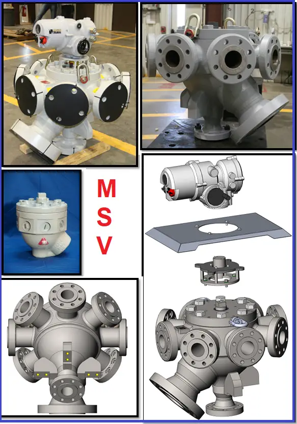
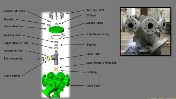
Rotary Selector Valve (RSV-Fig. 1) Components:

RSV Actuator
Heat Shield
Riser Kit
Thermal Coil
Thermal Blanket
Mounting Brackets
Lifting Pads

Applications:

A multiport valve can be used for fluid or gas systems

Multiple-port flow
Single port testing
Manual or automated operation
Water injection
Collection at the tank battery
Other-market application

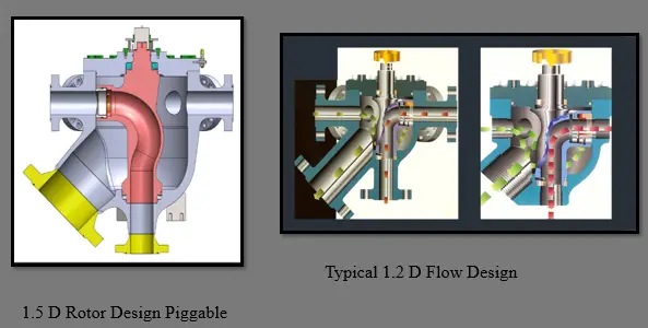
The RSV supports the capability of diverting multiple inlet ports, allowing each port to flow uninterrupted into a single chamber known as the body of the valve and out through a single group outlet port. A rotor stem, positioned in the center of the bowl, allows for the selection of a single inlet source to be diverted through a 1.2D or 1.5D flow line elbow and out through a single test outlet port.

The valve position is controlled by manual or automatic operation. Manual operation requires placing an indexing wrench directly on the outer stem of the rotor and rotating to the selected stopping position. The automatic operation uses a hydraulic, pneumatic, or electrical controller that attaches directly to the outer stem of the rotor allowing for local or remote positioning of the rotor to a selected port.

Advantages of Rotary Selector Valves

A rotary selector valve, also known as a rotary valve, is a type of valve used to control the flow of fluids or gases in a pipeline. It consists of a rotating cylinder that is divided into a series of compartments or ports. As the cylinder rotates, the ports align with the inlet and outlet ports, allowing the fluid or gas to flow through.

Rotary valves are commonly used in industrial applications, such as chemical and petrochemical processing, food and beverage production, and pharmaceutical manufacturing. They are preferred over other types of valves because they offer several advantages, including:

Low Maintenance: Rotary valves have a simple design and few moving parts, which makes them easy to maintain and repair.
High Durability: Rotary valves are made from materials that are resistant to corrosion and wear, which makes them durable and long-lasting.
Accurate Flow Control: Rotary valves offer precise control over the flow of fluids or gases, which makes them suitable for applications that require accurate dosing or metering.
Easy to Clean: Rotary valves are easy to clean and sterilize, which makes them suitable for use in sanitary applications.

Overall, rotary valves are a reliable and cost-effective way to control the flow of fluids or gases in industrial applications

Rotary Selector Valve Operation:

The RSV can be operated in a clockwise or counterclockwise direction.

As the rotor passes each port a spring-loaded wiper is engaged against the valve body to seal the seating surface. This creates a self-cleaning action and removes accumulated debris that might restrict proper operation. It also increases the life of the port seal and valve body.

An adjustable, spring-loaded Carbon Teflon Port Seal serves as a soft seal that prevents leakage at the test line and valve body junction. Back-up rings located on the port seal are designed to accommodate excess pressure, higher temperatures, or chemical presence.

Bidirectional Rotation
Self Cleaning
Self Sealing
Adjustable Sealing Surface
Back-Up Rings Improve Performance Life
Improved and Revised Metallurgy for Longer Life and Advanced Product Performance
Improved Elastomers and Seat Design to Meet Today’s Rugged Standards and Applications

Port Selection and Flow:

The Port Seal can be adjusted with a specially designed tool. The tool has two retractable spring-loaded pins that engage and disengaged via a pistol grip trigger. Each pin fits into a slot located on either side of the adjusting nut.

Specially designed O-Rings prevent external leakage through the valve body or head.

Emergency shutdown facilities; shut down upstream inlet ports in a single or group.

The downstream control valve can be remotely and automatically connected to the upstream setting point based on user requirements. The control system can be operated locally or remotely.

Optional quick disconnect fittings at all inlet/outlet flanges allow simple removal or relocation of the skid.

Special coatings for offshore or extreme conditions.

DESIGN CRITERIA:

ASME B16.34 (American Society of Mechanical Engineers)
ASME Sec. VIII, Div. 1 / Div. 2 (FCI- Fluid Control Institute)
ASME B16.5 (FCC-Fluid Catalytic Cracking)
NACE MR 0175 / ISO 15156 (National Association of Corrosion Engineers)
API 598 (American Petroleum Institute)
ANSI/FCI 70-2-2006 (American National Standards Institute)
MSS SP-55 (Manufacturers Standardization Society)
FEA Analysis, Proper Safety Factors, Industry/Local Required Codes
ASME VIII Division 1 Design Criteria

ANSYS finite element analysis software is employed for the main components of the RSV. Working and test conditions are analyzed and utilization factors (safety factors) to code allowable are verified.

A standard approach is to utilize the ASME VIII Division 1 design criteria and always employ the casting quality factor unless the design is unique, limited in quantity, and customized for specific applications.

Improvements to the RSV continue as the needs of the client base require with respect to metallurgy, flow, line-pigging characteristics, valve size, pressure classes, seals, differentials, controllers, communication protocols, and serviceability, metering capabilities, spill prevention or containment.

Additionally, we are faced with the task of ensuring each design supports ergonomic operation, safety, simplified integration, and environmental protection from leakages, such as H_²S fluids or gas.

Simplified Design – 3 Main Parts:

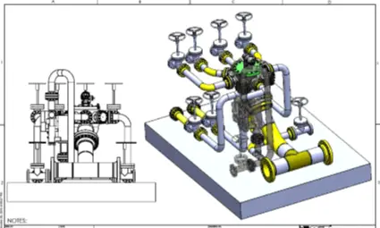
Skid Design:

Based on the results of the analysis conducted using FEA, the Sled meets the requirements of AISC with a safety factor greater than 1.5 for all loading conditions and a safety factor greater than 3 for the Lifting Eyes.

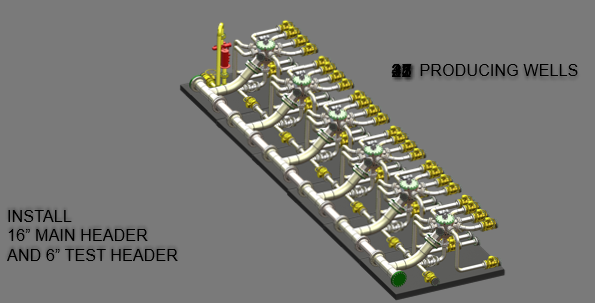
The multiport modular skid system utilizes a simple, design that saves time, money, and human resources. The system accommodates quick connect expandability for future field growth or quick disconnect to move those resources to other areas for improved utilization.

New Designs Based On Customer Requirements:

ANSI CL 1500 – 2500
SAG-D – Extreme Temperature
Full Body Alloy
Custom Skid – GA/Design

RSV SKIDS WITH A SINGLE FLOW METER:

Multi-Phase Flow Meter (MPFM)

A multiphase flowmeter is a device used in the oil and gas industry to measure the flow rates of a mixture of oil, gas, and water in pipelines. As the name suggests, it can measure multiple phases of a fluid flow simultaneously, which is important because, in many applications, the fluid stream is not homogeneous and can contain different types of fluids.

A multiphase flowmeter typically uses a combination of different technologies to measure the different phases of the flow, such as ultrasonic sensors, gamma-ray detectors, and differential pressure sensors. These measurements are then combined to calculate the flow rates of the individual phases.

Multiphase flowmeters are especially useful in offshore oil and gas production, where it is difficult and expensive to separate the oil, gas, and water before they are transported to shore. By accurately measuring the multiphase flow, operators can optimize production, reduce costs, and ensure compliance with regulatory requirements.

How does a Multiphase Flowmeter work?

The permanent multiphase flow meter (MPFM) uses technology for continuous flow rate measurements. The Typical Multi-Phase Flow Meter operates equally well in both oil and dry gas environments, making it possible to monitor and test dry gas, condensate, and oil wells with a single meter.

Via a remote data link to the multiphase meter, users can validate well data, perform quality control, generate well test reports, analyze well data, diagnose production, and interpret reservoir intervals. By eliminating the need for separators and their associated support systems or controls, the system is ideal for both Onshore and Offshore Applications, satellite, or unmanned locations, including subsea installations.

Since the need for a separator has been eliminated, the requirements for space, load, and maintenance are reduced. Continuous, highly accurate flow rate measurements allow for quicker response time to production anomalies. The typical MPFM has limited or no moving parts and is essentially maintenance-free. Remote monitoring increases the safety of field personnel and allows for better utilization of human resources.

Multiphase flowmeters (MPFM) work by measuring the different phases of a fluid flow, typically a mixture of oil, gas, and water, using a combination of different sensors and technologies. Here is a general overview of how an MPFM works:

Sensor Configuration: An MPFM typically consists of a combination of sensors that are placed in the flowline, including gamma-ray densitometers, ultrasonic sensors, and pressure transducers. Each sensor measures a different property of the fluid, such as density, velocity, and pressure.
Data Acquisition: The sensors are connected to a data acquisition system that collects the data from each sensor and processes it in real time.
Multiphase Flow Model: The data is then fed into a multiphase flow model, which uses algorithms and mathematical models to calculate the flow rates and properties of each phase of the fluid.
Output: The output from the MPFM can be displayed on a control panel or sent to a computer for further analysis. The information can be used to monitor the flow rates, the ratio of oil, gas, and water, and other important parameters.

Overall, the MPFM provides an accurate and reliable way to measure the flow of multiphase fluids, which is essential for optimizing production, monitoring the performance of wells and pipelines, and ensuring compliance with regulatory requirements.

Applications of MPFM

Multiphase flowmeters (MPFM) have a wide range of applications in the oil and gas industry, particularly in the upstream sector where they are used for the well testing and production monitoring. Here are some of the main applications of MPFM:

Well Testing: MPFM is used during the initial phase of well testing to determine the flow rates and characteristics of the fluids produced from a well. This information is used to optimize the production and recovery of oil and gas from the reservoir.
Production Monitoring: MPFM is used to monitor the production of oil and gas wells over time. This information is used to optimize the production process and to identify problems such as sand production, scale buildup, and water breakthrough.
Allocation Measurement: MPFM is used to measure the amount of oil, gas, and water produced from individual wells or fields. This information is used to allocate the production between different partners or to determine the royalties owed to the government.
Pipeline Monitoring: MPFM is used to monitor the flow of oil and gas through pipelines. This information is used to optimize pipeline operation and to identify problems such as pipeline corrosion, blockages, and leaks.
Reservoir Management: MPFM is used to monitor the behavior of reservoirs over time. This information is used to optimize the production process and to identify opportunities for enhanced oil recovery.

Overall, MPFM is a key technology in the oil and gas industry, allowing operators to accurately measure the flow of multiphase fluids and optimize production while minimizing costs and environmental impact.

Types of Multiphase Flowmeters

There are several types of multiphase flowmeters (MPFM) available in the market, each using different technologies and methods for measuring the flow rates of a multiphase fluid. Here are some of the most common types of MPFM:

Gamma Ray Densitometer (GRD): GRD uses gamma rays to measure the density of the fluid, which is then used to calculate the volumetric flow rate. This method is suitable for fluids with varying densities.
Venturi Meter: A Venturi meter is a type of differential pressure flowmeter that uses a constriction in the flowline to create a pressure drop. The difference in pressure is used to calculate the flow rate of the fluid. This method is suitable for low gas-liquid ratios.
Ultrasonic Flowmeter: An ultrasonic flowmeter uses sound waves to measure the velocity of the fluid. The transit time of the sound waves is used to calculate the flow rate of the fluid. This method is suitable for low liquid-liquid ratios.
Coriolis Flowmeter: A Coriolis flowmeter measures the mass flow rate of the fluid by detecting the Coriolis force that is generated by the fluid as it flows through a vibrating tube. This method is suitable for fluids with varying densities and viscosities.
Magnetic Flowmeter: A magnetic flowmeter measures the volume flow rate of a conductive fluid by inducing a magnetic field in the flowline and measuring the voltage generated by the flow of the fluid. This method is suitable for fluids with low conductivity.
Phase Doppler Anemometry (PDA): PDA is a laser-based method that measures the velocity of particles in the fluid flow. The velocity data is used to determine the flow rate and the size distribution of the particles in the fluid.

Overall, the choice of MPFM depends on the characteristics of the fluid being measured and the specific application requirements.

Multiphase Flow Meter Manufacturers

There are several reputed manufacturers of multiphase flowmeters (MPFM) in the market. Here are some of the top manufacturers:

Emerson Electric Co.: Emerson Electric Co. is a global technology company that offers a range of MPFM products, including Coriolis, ultrasonic, and gamma-ray densitometer flowmeters.
Schlumberger Limited: Schlumberger Limited is a leading oilfield services company that offers a range of MPFM products, including ultrasonic and gamma-ray densitometer flowmeters.
Weatherford International plc: Weatherford International plc is a multinational oilfield service company that offers a range of MPFM products, including ultrasonic and gamma-ray densitometer flowmeters.
ABB Ltd.: ABB Ltd. is a Swiss multinational company that offers a range of MPFM products, including Coriolis, ultrasonic, and magnetic flowmeters.
TechnipFMC plc: TechnipFMC plc is a global engineering and construction company that offers a range of MPFM products, including ultrasonic and gamma-ray densitometer flowmeters.
Krohne AG: Krohne AG is a German company that offers a range of MPFM products, including Coriolis, ultrasonic, and magnetic flowmeters.
Cameron International Corporation: Cameron International Corporation is a leading manufacturer of flow equipment, including MPFM products such as gamma-ray densitometer flowmeters.

These manufacturers have a long-standing reputation for quality and reliability and are widely used by the oil and gas industry for various applications.

Flow Characteristics:

The RSV can be operated in a clockwise or counterclockwise direction.
As the rotor passes each port a spring-loaded wiper is engaged against the valve body to seal the seating surface. This creates a self-cleaning action and removes accumulated debris that might restrict proper operation. It also increases the life of the port seal and valve body.
An adjustable, spring-loaded Carbon Teflon Port Seal serves as a soft seal that prevents leakage at the test line and valve body junction. Back-up rings located on the port seal are designed to accommodate excess pressure, higher temperatures, or chemical presence.

The RSV Multiport Skid provides a simple, cost-effective solution to manifold fluids in low maintenance, environmentally friendly package. The compact design reduces capital costs and allows for better utilization of resources when and where they are needed. The latest data communication technologies provide continuous feedback to help maintain a high level of operational efficiency and ensure quicker response time to production anomalies.

Process Engineering Deliverables for EPC of Oil and Gas Industries

Written by Anup Kumar Dey in Piping Interface,Process

Process Engineering Department is the main driver of any EPC Engineering Group. Because they provide information related to the actual process of what is going to happen. Other downstream departments use the information provided by the Process department in their design. The Process Department of any EPC organization normally generates the below-listed deliverables:

Process Engineering Deliverables

Process Engineering deliverables can be grouped into the following two classes:

Process engineering Documents, and
Process Engineering Drawings

Process Engineering Documents

The following deliverables come under the process engineering documents

Reports
Calculations
Information Packs
Data Sheets
Project Advice Note

Process Engineering Reports

Process Study Report
Basis of Design
Site Visit Report
Design Review Report
HAZOP Report
Design Review Closeout Report
HAZOP Closeout Report
Operating, Control Safeguarding Philosophy
Safeguarding Memorandum – update
EORD – update
Plant Operating Manual – update
Equipment List
Line List

Process Engineering Calculations

Separator Sizing
Pump Calculations
Relief Valve Calculations
Line Sizing
RO Sizing

Process Engineering Information Packs

Design Review Information Pack
HAZOP Review Information Pack
IPF Review Information Pack

Process Engineering Datasheets

Vessel
Control Valve
Pump
Storage Tank
Flare
Filter
Heater
Relief Valve

Process Engineering Drawings

PFS (Process Flow Scheme)/PFD (Process Flow Diagram)
PEFS/P&ID (Construction)
PEFS/P&ID (Demolition)
PSFS

What is Restrained and Unrestrained Pipes: Part 1

Written by Alex Matveev in Caesar II,Piping Stress Analysis,Piping Stress Basics,Start-Prof

Start-Prof is a part of PASS software suite for piping stress analysis, hydraulics analysis, boiler & pressure vessel, heat exchanger, column, tank design & stress analysis is available worldwide since 2018.

Article consists of 2 parts:

Part 1. Unrestrained, Totally Restrained and Partially Restrained Pipes. Bourdon Effect
Part 2. Restrained and Unrestrained Zones in the Buried Pipelines. Interpretation of Strength Criteria in ASME B31.4 and B31.8

ASME B31.4 and B31.8 codes divide pipes into restrained and unrestrained. Which part of pipe is restrained and which is not? Many engineers have a misconception about this. We will explain the difference and suggest new universal strength criteria, which cover both restrained and unrestrained pipes.

Before we begin, let’s say that actually, there are three types of pipe behavior instead of two described in ASME B31.4 and B31.8 codes:

Unrestrained
Totally Restrained
Partially Restrained

Unrestrained Pipe

Pipe Expansion from Cap Pressure Thrust Load

Unrestrained pipe expansion from the pressure load consists of two parts. The first part is the expansion due to the pressure load on the end cap. The second part is pipe shortening due to Hook’s law.

Pipe expansion from the pressure load on the end cap is:

L – Pipe Length

E – Modulus of Elasticity

Pipe cross-section area is

D – Pipe Outer Diameter

t – Pipe Wall Thickness

N – Axial Force in the Pipe

Axial force N is equal to the force acting on cap

P – Internal Pressure

Pipe expansion will be

Sh – Hoop Stress in the Pipe

According to Hooke’s law the axial deformation of the pipe under axial stress is:

v – Poisson’s Ratio

Pipe shortening due to internal pressure:

Total pipe expansion from pressure load is

If we add thermal expansion the equation will be:

– Temperature Difference between Installation and Operation temperature

– Coefficient of thermal expansion

Longitudinal stress caused by internal pressure is

If the left end is connected to pressure vessel nozzle or rotary equipment, then axial force in the equipment nozzle will be N as calculated above. But when equipment manufacturers calculate allowable loads, they assume that nozzle has end cap and vessel is under pressure. This means that axial stress caused by pressure is already included into allowable loads and should not be considered twice.

This means that we must exclude the pressure thrust load from axial force to calculate the support load that can be compared to allowable load on nozzle. To do this we must assume that pipe has two caps on the both ends. In this case the support load R will be equal to internal force N minus thrust force on the end cap, i.e. zero

A strength criterion for unrestrained pipe is:

Sallow ‑ Allowable stress.

If we add here bending stress and axial stress from loads other than pressure, we get

If we want to add torsion stress, we should calculate equivalent stress:

Allowable stress value depends on the code. Usually it is Sh or 0.75Sy for sustained loads, kSh or 0.9Sy for occasional loads, 0.9Sy…Sy for test state. Occasional load factor k=1.15…1.8 depends on selected code. Sy is yield stress, Sh – code allowable stress at operating temperature.

Thermal expansion has no effect on unrestrained piping systems, i.e. this equation usually used for sustained and occasional stress check in piping systems from pressure, weight and other force-based loads.

The code equations were created for manual calculation. But now most of pipe stress analysis software can consider Bourdon effect. This means that code equations should be modified to match the current level of technology.

If axial force N is calculated using software that considers Bourdon effect, then we should subtract PD/4t value from axial force otherwise it will be included twice:

The criteria for software analysis where M and N calculated with Bourdon effect should be just:

This has been already done in ASME B31.3 for Process Piping, GOST 32388 for Process Piping, GOST 55596 for District Heating Networks, SNiP 2.05.06-85 for Gas and Oil Pipelines, but still not fixed in all other ASME B31.X and EN 13480 codes.

Totally Restrained Pipe

For a restrained pipe with two anchors on both ends, thermal expansion should be zero

The axial force required to compress the pipe back to its original length can be calculated from this equation:

Therefore support load should be:

After substitution the thermal expansion equation we got final support load for restrained pipe:

The value of axial force can be obtained from the equilibrium conditions near the anchor. Axial force is equal to reaction in anchor minus the pressure thrust force that is received by anchor and doesn’t acting on the pipe:

Final equation for axial force in restrained pipe is

Axial stress in the restrained pipe will be

A strength criterion for totally restrained pipe is:

If we add here bending stress M/Z and axial stress N/A from loads other than pressure, we get

If we want also consider torsion and hoop stress, we should use the equivalent stress equations like described for unrestraint pipes.

If axial force is calculated using software that considers Bourdon effect, then we should subtract pressure axial stress:

The criteria for software where M and N calculated with Bourdon effect and thermal expansion should be:

A criterion is the same as for unrestrained pipes, but allowable stress is usually 0.8Sy…1.0Sy to prevent the Yielding through all pipe length.

The maximum temperature difference for fully restrained pipe, ignoring longitudinal buckling effect, can be found by equation:

If pressure is zero, this value is about 80…110 C for steel pipes.

Partially Restrained Pipe

If we add flexible spring instead of rigid anchor on the right end of the pipe, we will get the third pipe condition – partially restrained.

We will pass the derivation of equations process and just show the final equations in table below.

The strength criteria for partially restrained pipes should be

From sustained primary loads:

From occasional primary loads

From both primary and secondary loads acting simultaneously

Primary Loads – are force driven not self-limiting loads like weight, pressure, relief valve thrust, wind, etc.

Secondary Loads – are displacement driven self-limiting loads like thermal expansion, anchor movements, support or soil settlement, etc.

Unrestrained and fully restrained pipe conditions can be easily calculated manually, but third condition require using of pipe stress analysis software, because spring stiffness k depends on connected pipes.

Bourdon Effect Model in PASS/Start-Prof

Now I will explain how PASS/Start-Prof software considers pressure Bourdon effect in arbitrary piping model. Start-Prof model the pressure loads consist of two parts.

Firstly, Start-Prof adds pressure thrust force on each end of the pipe.

Secondly, Start-Prof adds axial deformation for each pipe. It equal to pipe thermal expansion minus pressure shortening.

The combination of these two loads allows to model correctly any type of piping: unrestrained, restrained, and partially restrained.

Bourdon effect makes a significant contribution to the support loads, displacements, and stresses for

High pressure piping
Plastic piping (PE, PP, PB, PVC)
FRP/GRP/GRE piping

Start-Prof always preforms analysis with Bourdon effect, it is non-disabling function.

Refer Part 2 for next part…..

10 Considerable Points for Pressure Vessel Nozzle Load Tables

Written by Anup Kumar Dey in Caesar II,Mechanical,Piping Interface,Piping Stress Analysis,Piping Stress Basics

Every EPC company must have project-specific pressure vessel nozzle loading tables which are used for comparing allowable nozzle loads for vessels, columns or towers, heat exchangers, Drums, or any similar type of equipment. Normally forces and moments at the nozzle and shell interconnection are provided in a tabular format. These force and moment values are decided based on the following major factors:

Nozzle diameter
Connected flange rating
Equipment and nozzle thicknesses.
RF Pad thickness if any
Equipment diameter, etc.

Using these tables is quite simple. However, we must keep in mind a few points while using those tables. This article will list those important points for using these tables easily.

1. Before checking the tables, find out the load and moment directional drawing from which we have to correlate the Caesar II axis.

2. Each nozzle, including those designated “spare” but with the exception of man-holes and instrument nozzles shall be designed to withstand the forces and moments specified herein. The indicated loads are to be considered to act at the shell/head-to-nozzle intersection.

3. For nozzles matching with any global direction (other than head nozzles) compare the values mentioned on the tables with global force values in CAESAR II output.

4. For inclined nozzles in the horizontal plane (with respect to any global direction) there are 2 options as listed below.

Compare loads mentioned in the tables above with local element forces in CAESAR II output. In that case, the local X force will be a radial force and compare other directions to get proper forces.
Otherwise rotate the CAESAR II input model to match the nozzle axis with any global Caesar II axis and compare the loads and moments.

5. For Head nozzles (nozzle axis and equipment axis same direction) compare M_x and M_z as per √[{(M_x)²+(M_z)²}] ≤ √[{(M_L)²+(M_C)²}]

6. In the case of any vessels in the packaged area, these values shall not be applicable and nozzle loading shall be coordinated with the vendor.

7. In the case of any licensor / proprietary item, these values shall not be applicable and nozzle loading shall be confirmed by them.

8. Allowable for self-reinforced nozzle shall be more than as mentioned in the above table. In that case, allowable shall be exercised from the vendor.

9. For jacketed nozzles, loads are to be confirmed by the vendor.

10. These tables are not applicable for checking loads at flange faces.

Few more Resources for you..

A short Presentation on Basics of Pressure Vessels
Brief Explanation of Major Pressure Vessel Parts
A Presentation on VESSEL CLIPS or VESSEL CLEATS
Understanding Pressure and Temperature in the context of Pressure Vessel Design

Online Course on Pressure Vessels

If you wish to learn more about Pressure Vessels, their design, fabrication, installation, etc in depth, then the following online courses will surely help you:

Pressure Vessel Design Masterclass – ASME VIII

Pressure Vessel Fabrication -Mechanical Engineering, Oil&Gas

Master In Pressure Vessels Heads in Hindi

AFT Impulse Pulsation Frequency Analysis (PFA) Module

Written by Anup Kumar Dey in Mechanical,Piping Interface,Piping Stress Analysis,Process

This presentation is prepared by Mr. Deepak Sethia who is working in ImageGrafix Software FZCO, the Hexagon CAS Global Network Partner in the Middle East and Egypt. He has extensive experience in using Caesar II, PV Elite, AFT Impulse software, and troubleshooting. The points that will be covered in this article are:

Introduction
Natural Frequency and Resonance
Piping System Vibration and Resonance
PD Pump Pulsation
Overview of PFA for Impulse

Piping System Vibration and Resonance:

Piping systems can vibrate or resonate in two ways

– Through the pipe solid material

This is called “mechanical vibration”
If the vibration frequency is at the natural frequency it is called “mechanical resonance”

– Through the fluid inside the pipe

This is called “acoustic vibration”
If the vibration frequency is at the natural frequency it is called “acoustic resonance”

PFA PROCESS IN AFT IMPULSE:

PFA Process:

Build the model

– This model represents the suction side of a system with two PD pumps (J8 & J9) in parallel fed by a centrifugal pump (J1)

– We will analyze the upper PD pump (J8)

Select Pulsation Setup from the Analysis menu

▪ This is where the “ring” will be defined

– Specify junction (only one in the system) and pulse start time

– The automatic magnitude of the strike will be twice the steady-state flow

Details of the PD pump are entered on the PD Pump Setup tab

– Used to generate the flow vs. time pump curve for the child pump scenarios

With everything defined we can view the flow pulse that will be used to “ring” the system

– Click Show Pulsation Graphs… in the lower-left corner

The pulse spike and the FFT of the pulse without filtering are shown in the first two tabs

Once the low-pass filter is applied (140 Hz in this case), the pulse spike is now a decaying sine wave

Evaluate Frequencies:

After running the model, go to the Graph Results window
Select the new Frequency tab
Select the pipe location(s) to analyze and click Generate
- The spikes show the frequencies that excite the system at that location

Right-clicking on the annotation brings up a menu, allowing the user to Evaluate Excitation Frequency

For PD pumps, the speed (RPM) will be determined at that frequency for the harmonic multiples

– A red dot appears indicating the frequency is being evaluated

These scenarios have special properties since they are dependent on the configuration of the parent scenario

They are read-only so most of the model cannot be changed
- They will be deleted when the parent is changed
- They are named with the pump speed and frequency

Analysis:

When the model is run, there will be several blocks of time steps used to determine when the model reaches an equilibrium– This eliminates any artificial fluctuations caused by the PD pump flow, and leaves just the steady-state harmonics of the system

Graphical Report:

The frequency response graph can again be generated– Notice the spike occurs at the frequency of interest.

Output Report:

At the end of the run, the maximum peak-to-peak pressure levels are checked against the API-674 standard

– If the levels are OK there will be a confirmation

– A warning is given if there are locations that exceed the maximum set by the standard. It will list the location where the largest DP occurred.

Generate the Force file for CAESAR-II:

Elevated Flare systems used in Process Industries

Written by Anup Kumar Dey in Mechanical,Piping Interface,Process

What is an Elevated Flare System?

The elevated flare system consists of a flare header, a knock-out drum, and a flare stack. The waste gas and condensate are collected from the whole plant through the flare header and then the condensate is separated in the knock-out drum finally, the gas is burnt in a stack at a high elevation. As the combustion of gases (toxic) is done at the flare tip at a high elevation, the complete system is called Elevated Flare System.

Purpose of flare system

The primary function of a flare system is to use combustion to convert flammable, toxic, or corrosive vapors to less objectionable compounds like CO₂.

Why not cold vent instead of flaring?

Methane is roughly 30 times more potent as a heat-trapping gas than CO₂. Hence cold venting of HC gases is not allowed as per pollution control board directives.

Design standards for Flare System

API 521: Pressure-relieving and Depressuring systems
DEP 80.45.10.10: Flare and vent systems (amendments to API 521)
API537: Flare details for refinery and petrochemical service
DEP 80.45.11.12: Flare details (amendments to API 537)

Types of Flares (Fig. 1)

Elevated flares: Commonly used in the oil and gas industry and the most economical.
Enclosed flares: Used in plants where a visible flame is not acceptable. Also used for offshore facilities.
- Advantages: Low noise and radiation levels;
- Disadvantage: Poor dispersion of gases during flameout condition (flare needs to be tripped on gas detection)
Ground flares: Used for liquid or two-phase relief flaring.
- Advantages: Low radiation, low noise;
- Disadvantage: accumulation of vapor cloud, high initial cost.

Types of Elevated Flares (Fig. 2):

Self-supported stacks

Simplest and most economical design; Stack height up to 100 ft overall height; As the flare height and/or wind loading increases, the diameter and wall thickness required become very large and expensive.

Guy wire-supported stacks

Most economical design in the 100- to 350-ft height range. Normally, sets of 3 wires are anchored 120 degrees apart at various elevations.

Derrick supported stacks

The most feasible design for stack heights above 350 ft. Derrick supports can be fabricated from pipe (most common), angle iron, solid rods, or a combination of these materials. They sometimes are chosen over guy-wire-supported stacks when a limited footprint is desired.

Non-Assisted / Assisted Flares:

Non-assisted flares are the flares that do not use any assist media and are typically used for hydrocarbon or vapor streams that do not cause smoking (i.e. For clean-burning gases like methane, hydrogen, carbon monoxide, ammonia, hydrogen sulfide) or when smoke is not a consideration.
The incomplete combustion of heavy HC gases produces Carbon monoxide, which is the main component to create smoke. For flaring heavy gases, a smokeless operation can be achieved by assisting media such as steam, air, or gas which improves the mixing of flare gas with air.
Steam-assisted flares (Fig. 3) for smokeless operation. Steam increases the momentum of flare gas which enhances fuel-air mixing leading to complete combustion. Also, the water-gas shift reaction converts CO to CO₂

CO + H₂O ⇌ CO₂ + H₂

Air-assisted flares (Fig. 3) are used where smokeless burning is required. It is used when steam is not available or where low-pressure air delivery offers a lower cost. (the only fraction of the requirement of air is mixed with flare gas to promote momentum which effectively entrains additional combustion air from the surrounding).

Steam Assisted and Air Assisted Flares — **Fig. 3: Steam-Assisted** and Air-Assisted Flares

Flare load estimation (Fig. 4)

**Fig. 4: Example of Flare Load Estimation**

Fire zone: Wetted areas within a 300 m2 (3200 ft2) plot area shall be considered when a system’s relief loads are calculated.
Flare gas flow rate: Tip diameter is decided based on the design flow rate.
Mach number in Stack: 0.5
Mach number in tip: 0.5 to 0.8 (depends on allowable pressure drop)
Lower gas velocity (Fig. 5): When the gas flow is so low that the local gas velocity is less than flame velocity, air entrains into the flare tip leading to burning back / flashback. At very low gas velocities, the flame can travel back through the mixture (flashback) into piping and KOD.

**Fig. 5: Effect of Lower and Higher Gas Velocity**

Higher gas velocity (Fig. 5): When the gas flow is higher than the design capacity, then the local gas velocity becomes higher than the flame velocity leading to detached flame or flameout (higher velocity leads to turbulence, which in turn reduces HC component concentration below LFL)
Flame velocity: The burning velocity or flame speed is the velocity at which a flame front moves through the unburnt gas/air mixture. This flame speed varies with the air/gas mixture ratio and the chemical makeup of the gas.
Purge gas requirement: To avoid air ingress down the flare stack purge gas is injected in the flare header. The injection rate should be controlled by a fixed orifice, rotameter, or other devices that ensure the supply remains constant and is not subject to instrument malfunction or maladjustment.
Purge reduction seals (Fig. 6): To reduce the purge rate purge reduction seals are used.

Liquid seal

The liquid seal drum shall be designed as a pressure vessel with a design pressure of at least 7 bar (100 psig) to maintain containment against internal deflagration.

Where there is a risk of an obstruction in the flare due to process flows creating an ice plug with the liquid seal, alternate sealing fluids such as a glycol/water mixture (60% EG & H2O freezing point –45 deg C) or other means to prevent freezing SHALL [PS] be implemented.

For LNG facilities, liquid seal drums shall not be used, since in the event of a cold release this may form an obstruction in the flare relief system.

Allowable Liquid droplet size (to avoid burning rain): Burning rain occurs when the rate of burning (depends on the type of flare) of liquid droplets is lower than the rate of settling of droplets (depends on droplet size).

Drift distances of burning liquid droplets from an inadequately designed flare system can be considerably greater than 200 ft (60 m).

If the liquid is not drained from flare gas, at a gas velocity of 3-4 m/s – liquid droplets of 1000 microns can be entrained which can cause burning rain in the flare.

Liquid droplet size allowed without burning rain

Unassisted flares: <600 micrometer
Steam or air-assisted: <600 micrometers (less than 1% mass)
High pressure (if operated at least 200 kPag): <1000 micrometer (less than 1% mass)

Flare Knock Out Drum (KOD)

Design pressure of KOD:

5 barg (50 psig) when a liquid seal drum is located between the KO drum and a flare stack.
7 barg (100 psig), if there is no liquid seal drum in the system.

For a multi-process unit facility (e.g., refinery) based flare KO drum where it may not be immediately clear which unit is sending liquid to the flare, liquid space on top of LA (HH) SHALL [PS] be designed to contain the maximum emergency liquid relief rate from the largest single contingency for a period of at least 15 minutes for the unit KO drum and at least 20 minutes for the flare KO drum, without taking credit for pump out capacity.

Flare Height

The height of the flare (Fig. 7) is established based on allowable thermal radiation levels. Flare height depends on the available plot and the distance of nearby equipment from the flare stack.

More plot area: Low flare stack height
Less plot area: Higher flare stack height

**Fig. 7: Flare Height vs Available Plot Area**

Thermal radiation:

The effect of thermal radiation on a person at grade or at an elevated platform shall be checked by radiation calculation.

Thermal Radiation affects human skin (skin burn).

Exposure Times Necessary to Reach the Pain Threshold

31 kW/m2 – Up to 20 s
15 kW/m2 – Up to 1 hour
58 kW/m2 – Continuous

If personnel exposure to radiant heat exceeds the guidelines provided, then shielding should be considered.

Depending on the location the thermal radiation limit is provided in Fig. 8

The solar radiation need not be added to calculated thermal radiation values (0.79 to 1.04 kW/m2) from the Flare.
A wind velocity of 10 m/s (22 mph) at the elevation of the flare tip, blowing towards the receiver, is a typical assumption for flame tilt assessment.
When two flares are located in close vicinity, combined radiation effects shall be calculated.

Dispersion Analysis

To ensure safe operation during periods when the flame might have extinguished, the concentration of hazardous components should be determined using dispersion analyses, assuming the flare is functioning as a vent only.

Level of Concern	Hydrogen Sulphide (Concentration, Time)	Sulphur Dioxide (Concentration, Time)
8 Hour TWA (Threshold Limit Value)	5 ppm, 8 hours	2 ppm, 8 hours
15 Minute STEL (Short-Term Exposure Limit)	10 ppm, 15 minutes	5 ppm, 15 minutes

Short-term exposure limits (STELs) are set to help prevent effects, such as eye irritation, which may occur following exposure for a few minutes

Smokeless requirement

Local rules and regulations shall be followed. Typically flare combustion quality shall meet Ringelmann Index 1 criteria (Fig. 9).

Smokeless flowrate shall be the normal flow that is expected in day-to-day operations. Do not specify the design capacity for smokeless operation.

A scale used to define levels of white, gray, and black i.e. intensity of smoke

Ringelmann No. 0 is clear smoke
Ringelmann No. 5 is 100 percent black.
Ringelmann No. 1 is equivalent to 20 percent black

Other requirements

Noise: For normal flow rate (including starting-up and shutting-down): 85 dB(A) at the sterile radius. For emergency conditions: 115 dB(A) at sterile radius
Combustion efficiency: greater than 98%
The number of pilots (Fig. 10): The number of pilots required is a function of the flare burner diameter. For very small flares, a single pilot will reliably light the flare gas. However, it should be noted that if only a single pilot is used, a single pilot failure would represent a complete failure of the ignition system. Recommended installing at least 2 pilots for tip size of up to 8″ to increase reliability. As the flare burner diameter increases, the number of pilots required to reliably light the flare, regardless of wind direction, increases.

Flare gas recovery system Safety considerations

Path to flare: PRVs, depressuring systems, etc., shall always have flow paths to the flare available at all times.
Reverse flow: Because flare gas recovery systems usually involve compressors that take their suction directly from the flare header, the potential for the reverse flow of air from the flare into the compressors at low flare gas loads shall be considered.
Monitor oxygen content in the flare header and provide recovery system trips. Provide a low-pressure trip on the recovery system suction to avoid air ingress. Liquid seal drum (not practical in AP flare systems)

Few more useful Resources for you…

Pre-Commissioning and Commissioning Checklist for Flare Package
Routing Of Flare And Relief Valve Piping: An article-Part 1
Flare systems: Major thrust points for stress analysis
Stress Analysis of PSV connected Piping Systems Using Caesar II
Articles related to Process Design
Piping Layout and Design Basics
Piping Stress Analysis Basics

Recent Posts