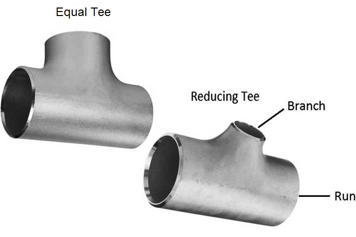
Piping Tees are used either for dividing the main fluid flow into two streams or for combining flow from two streams. The term Tee for these types of pipe fittings most probably comes from the resemblance of the English letter Tee.
The main run pipe has often termed a Header and the other as a branch. The branch size may be smaller or equal to the run pipe size but it cannot be larger. Tees having branch size equal to run size are called equal tees & others as unequal tees or reducing tees.
Tees are normally designed based on ASME B16.9 or ASME B16.11. Tee is always normal or perpendicular to the pipe axis and is normally produced by forging.
Types of Piping Tee Connections
Piping tee connections are classified according to the branch size and end connection.
Based on the branch size, there are two types of piping tee connections. They are:
Equal Tee, and
Reducing Tee
Equal Piping Tee:
When the branch size is equal to the run pipe it is called Equal Tee pipe fitting.
Reducing Piping Tee:
In the case of reducing tee, the branch size is smaller than the run pipe size. there is a limitation to the branch size. It can not be sufficiently smaller. For example, Reducing Tee from 16″ pipe is available up to 6″ branch size. 16″ X 4″ piping tee is not manufactured. Usually reducing piping tee connections are manufactured till a branch pipe size of one size lower than 1/2 the parent pipe size. This rule is valid till 28″.
Fig. 1: Equal Tee vs Reducing Tee
Based on the pipe end connections, tees are classified as follows:
These are usually forged and used up to 2” run size on services where socket welded connections are permitted.
The applicable dimensional standard is ASME B16.11 and material standards including ratings are the same as those for socket-welded elbows.
Normal industry practice is to use socket welded tees up to 1 1/2” run size.
Screwed-end Tees
Their use including rating, dimensional, and material standards are the same as applicable to screwed elbows.
Butt welding Tees
The dimensional standard applicable for equal and unequal tees is ANSI B16.9. These are available from 1/2” through 48”.
Unequal butt welding tees are available having branches up to one size lower than half run size e.g. If the run size is 8”, unequal tees are available in sizes 8” × 6”, 8” × 5”, 8” × 4” & 8” × 3 1/2”.
Applicable Pressure temperature rating and material standards are the same as those for butt-welding elbows.
Butt welding tees are usually used for size 2” and above and in smaller sizes for services where the use of socket weld joints is prohibited.
Flanged Tees
Their use including pressure rating, and dimensional & material standards are the same as applicable to flanged elbows.
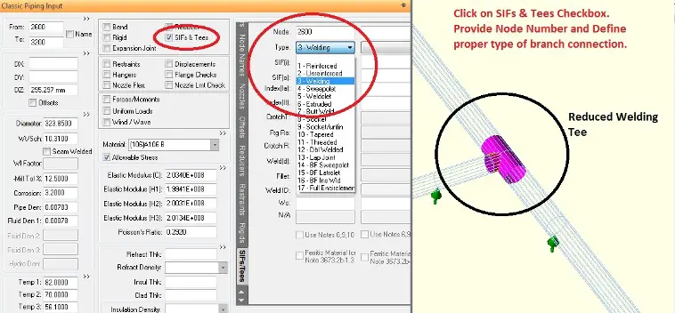
In normal large-bore pressure piping most often Butt-welded Tee connections are used. The ASME B31.3 (Appendix D) is used to provide a formula for calculating the SIF value at tee connections which Caesar automatically calculates when Tee is defined. From the ASME B31.3-2020 onwards, Appendix D is deleted from the code. Now Stress Intensification and Flexibility factors are to be calculated using the ASME B31J code. The Tee connections are normally defined in Caesar as shown in the attached figure.
Fig. 2: Tee modeling in Caesar II
For pipeline systems, a special type of tee is used, known as Barred Tee.
Piping Tee Dimensions
Equal Tee Dimension Chart
Refer to the following table (Table-1) for the Tee dimension chart for equal pipe tee as per ASME B16.9
NPS (Inches)
Outside Diameter at Bevel (D, mm)
Center to End (C, mm)
Center to Center (M, mm)
1/2
21.3
25
25
3/4
26.7
29
29
1
33.4
38
38
1 1/4
42.2
48
48
1 1/2
48.3
57
57
2
60.3
64
64
2 1/2
73.0
76
76
3
88.9
86
86
3 1/2
101.6
95
95
4
114.3
105
105
5
141.3
124
124
6
168.3
143
143
8
219.1
178
178
10
273.0
216
216
12
323.8
254
254
14
355.6
279
279
16
406.4
305
305
18
457.0
343
343
20
508.0
381
381
24
610.0
432
432
26
660
495
495
28
711
521
521
30
762
559
559
32
813
597
597
34
864
635
635
36
914
673
673
38
965
711
711
40
1016
749
749
42
1067
762
711
44
1118
813
762
46
1168
851
800
48
1219
889
838
Table 1: Equal Pipe Tee Dimensions
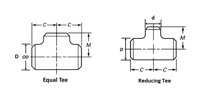
Refer to Fig. 3 below to understand the notation used in Table 1 and Table 2.
Fig. 3: Equal Tee and Reducing Tee Nomenclatures for Pipe Tee Dimensions
Reducing Piping Tee Dimensions Chart
Refer to Table-2 which provides the reducing Pipe Tee dimensions.
Awareness of Safety Rules during a Field Visit (Operating site/Construction Site) is a must. But most of the new designers/engineers working in design consultancy firms are unaware of it. While making a field visit to a chemical process unit whether it be an upstream oil and gas processing installation, a refinery, or a petrochemical plant, safety rules need to be strictly followed. This article explains some basic safety rules for a site visit. Readers can suggest additional points to be taken care of during the field visit.
Carry your own Personal Protective Equipment (PPE)
It is suggested to carry your own personal protective equipment (PPE). Even though these may be available at a few sites but still do not expect the same. Carrying your own PPE has its own advantages like fitment and personal hygiene. It may not be possible to get PPE items of the perfect size and you may not feel comfortable wearing used PPE items.
Complete Mandatory Safety Training prior to Site Visit
Before the field visit, check if there is a requirement to finish some mandatory safety training. If so, attend those before planning for site-visit. For example, a one or two-day course on oil-field safety and Hydrogen Sulfide Safety and exposure protection has to be taken up and a certificate of completion be obtained as a mandatory requirement for many upstream oil and gas companies prior to the field visit.
Check regarding additional Safety Precautions from Plant Operating Staff
It is always better to enquire about the safety precautions of the operating plant from the operating staff. Also, while entering the chemical process unit premises for the first time ensure that the plant operations staff accompanies and guides you. Learn about the layout of the plant and any special safety precautions to be considered from them. Entering an operating area without any awareness of what is around you is dangerous and foolhardy.
Follow Plant Safety Sign Boards thoroughly
Almost all operating plants provide safety signboards inside the plant to make you aware of safety details. So, Lookout for such signboards when walking around the plant or unit.
Be Attentive while walking on elevated platforms
When walking on elevated platforms ensure that you are attentive and looking all around to see where you are landing your feet. Pay attention that your head is not bumping against a beam or piping. Be extra careful as there may be open grates or hatches for maintenance work to avoid a falling accident.
Avoid Touching valves, pipes, or instrument surfaces by Barehand
If you are not authorized, Do not touch valves or instruments with barehand. Without knowing the fluid content in the pipe, If you touch bare pipe or valves, Burning can happen. Even solar radiation on a bare pipe can cause the surface temperature to be high enough to cause 1st-degree burns and blisters.
Seek help from Site operating Staff for Data measurement
Always ask the operating staff to collect the required field data. In case, you are required to take site readings from field instruments ensure that you have a proper foothold and can walk around the instrument without obstruction. Be extra cautious while climbing monkey ladders and do it very carefully and slowly.
Avoid Dehydration
Always keep yourself hydrated and carry water with you. Normally it is required to work in the open sun for quite some time, So make sure that you have taken plenty of fluids before walking around. Dehydration can cause dizziness and lack of focus which could lead to an accident. If you are unwell, it is not advisable to undertake a field visit.
Avoid Removing your PPE
Do not remove your Personal Protective Equipment kit just because you are feeling sweaty and itchy while working in hot and humid conditions in the plant area where PPE is mandatory. In case it is required, take a break in a safe convenient place where you can remove your PPE to recompose yourself before going back to work.
Avoid changing any set points when inside the control room
Do not change any setpoints of the process control instruments while sitting in the control room unless you are both authorized and know the consequences of your actions in terms of the effect on the process.
Know about emergency Exits and Gathering Points beforehand
Before entering the plant premises make sure that you are briefed about the emergency exits and gathering points by the operations staff of the plant. Pay utmost attention to what is being told to you.
No Smoking or Eating inside plant premises
Needless to tell that it is not allowed to smoke and eat in the plant premises except for areas designated for smoking and having food/beverages.
There could be many other points for a safe field visit and I request the readers to contribute some more points for a safe and successful field visit in the comments section.
Plant Design Management System or PDMS is one of the most widely used engineering design software in the 3D CAD industry for developing or designing plants. UK based MNC AVEVA developed this software.
Why is PDMS is popular?
PDMS is highly popular in plant design because of its various benefits like
Customization is very easy.
It can be used by many users and multi-discipline together. The software allows engineers and designers at various locations to create, control and manage project changes simultaneously.
It can be used for engineering, design and construction projects in offshore, onshore oil & gas and chemical industry.
It has in-built modules for the design of piping, ducting, equipment, structure and cable trays.
Its colourfull 3D environment is awesome.
It has inbuilt tools that ensure the clash-free design
It can handle big projects with ease, without error.
Professionals using PDMS
On a broad scale PDMS software is used by the following professionals:
Piping Professionals i.e Engineers and Designers
Civil Engineering Professionals
Draftsmen from all disciplines
Chemical Engineering Professionals
Petrochemical Engineers
Designers involved in the 3D design process
Students and Professionals from the Mechanical engineering domain.
In this article, I will share a few collected PDMS video tutorials to help beginners. To learn from these tutorials you must have to install the PDMS software on your PC or laptop.
PDMS Tutorial/ Lesson 1. Creating Equipment
In this lesson, you will learn how to create equipment through primitives and matching two surfaces by the ID point method and learn simple object moving commands.
Tutorial/ Lesson 2. Measuring Distance
In this lesson, we will discuss different types of measuring methods; element to element and graphic to the graphic.
HOW TO MEASURE DISTANCE
Tutorial/ Lesson 3. Creating Nozzle
In this lesson, we will learn how to create a nozzle on a vessel and a tank and how to create any type of hole by negative primitives.
HOW TO CREATE NOZZLE AND CREATE HOLE BY NEGATIVE PRIMITIVES
Tutorial/ Lesson 4. Offsetting & Rotating a Nozzle
Offsetting and rotating nozzles are very important in piping design. In this lesson, how to rotate and offset nozzles is explained thoroughly through various commands.
This video will explain how to rotate, offset & mirror the equipment in PDMS.
HOW TO MIRROR, OFFSET & ROTATE EQUIPMENT
Tutorial/ Lesson 6. Modifying Equipment & Nozzle
This video tutorial is prepared with an aim to help you learn how to modify equipment & nozzles and adjust parameters accordingly.
HOW TO MODIFY EQUIPMENT & NOZZLE
Sample PDMS Project
Tutorial/Lesson 7. Creating Equipment (Heat Exchanger, Air Cooler, Vessel or Pump)
In this lesson, we will learn how to create air cooler, heat exchanger, vessel & pumps.
HOW TO CREATE STANDARD EQUIPMENT
Tutorial/ Lesson 8. Modifying Equipment according to Construction Drawing
In this lesson, we will learn how to modify standard equipment. But in this video, you will see specifically how to modify a centrifugal pump. In a similar way, you can easily modify other equipment.
HOW TO MODIFY STANDARD EQUIPMENT ACCORDING TO CONSTRUCTION DRAWING
PDMS Tutorial/ Lesson 9. Creating Single Branch-Piping Modelling
In this lesson, we will learn how to create a single branch connection.
In this video,, we will learn how to create a structure beam & column. and how to extend beam & column by a different method and how to copy-paste the floor.
To bring the constructed/installed system to deliver the desired function.
Pipeline commissioning means introducing crude/ product/Gas in the pipeline from originating station, filling the entire length, and then start delivering to the receipt system.
What do we need prior to commissioning?
The pipeline and associated facilities are completed in all respect
All Fire and Safety equipment/facilities are tested and commissioned
Availability of dedicated communication
Statutory Clearances obtained
Availability of Product (HSD)/ Crude oil – Not less line-fill
Required Manpower is placed at all locations
Availability of water and its disposal plan
Availability of a dedicated commissioning team
Critical issues in commissioning a Petroleum Pipeline
The movement of hydrocarbon in an empty pipeline can generate static current.
Hydrocarbon Vapor mixed with oxygen may lead to an explosion.
There may be the formation of an Air / Vapor pocket that may get compressed leading to a rise in pressure.
Air/vapor pocket may explode in the receiving tank leading to damage to the tank roof seal.
Leakage of any hydrocarbon may lead to fire or damage to the environment.
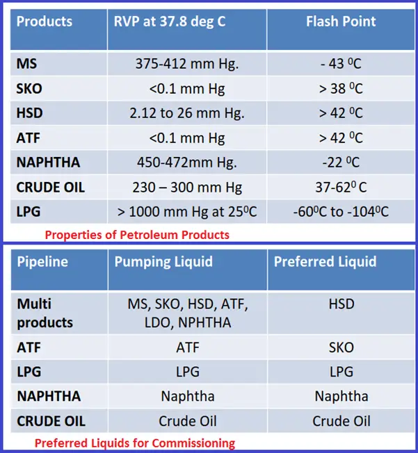
Properties of Hydrocarbons
Flash Point:-The flash point of a volatile liquid is the lowest temperature at which it can vaporize to form an ignitable mixture in air.
Vapor Pressure:-The vapor pressure of a liquid is the pressure exerted by its vapor when the liquid and vapor are in dynamic equilibrium. At a given temperature, a substance with higher vapor pressure vaporizes more readily than a substance with lower vapor pressure.
Properties of Petroleum Products and Preferred Liquid for Commissioning:
Fig. 1: Properties of Petroleum Products
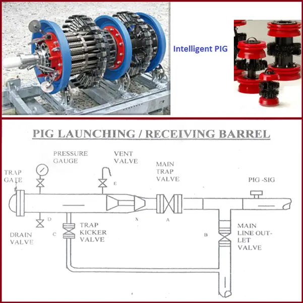
What is a PIG?
A device that moves through the inside of a pipeline for the purpose of cleaning, dimensioning, sealing, and inspecting.
Check dents, buckles, and any other internal abnormalities
To minimize interface generation between two dissimilar products
To avoid cross‐contamination
To evacuate the pipeline
Conventional / Utility Pigs – Different types
Various components are fitted on a mandrel.
It can be uni‐directional or bi‐directional
Fig. 2: PIG and PIG Launching Barrel
Intelligent Pig (Fig. 2)
To record bends, dents, ovality, bend radius & angle.
PIG Launching / Receiving Barrel: Refer to Fig. 2
Commissioning of a Gas Pipeline
A gas pipeline is treated as Tank. However, before taking gas in the Pipeline, it is to be made moisture and oxygen-free.
Commissioning Steps
Drying – Purging of super dry air: Compressed Super dry air is purged using air compressors with accessories viz. Moisture Separator, Oil Separator, and Dryer. The air shall be supplied in the pipeline at (-) 20 deg. C dew point. Super dry air with dew point (-) 20 deg. C will have sufficient capacity to absorb water vapor to the extent of 30 % of the desired capacity.
Vacuum Drying: The process utilizes a high-capacity vacuum to reduce pressure within the Pipeline to a level from 760 Torr to 40 Torr. At this pressure (40 Torr), any water within the pipeline will start boiling and vaporizing. Air left inside the Pipeline is subjected to a vacuum of 40 Torr, and the water vapor will expand approx. 18.8 times, which will be displaced using high-capacity vacuum booster pumps (rated capacity 5000 CuM/Hr)When the vacuum of 7.6-10 Torr is achieved, it is confirmed that the whole pipeline system has been dried to the required level.
Nitrogen Purging: At vacuum level 7.6 Torr and dew point (-) 20 deg.C, the oxygen content inside the Pipeline is 0.20%. To further dilute the oxygen content, nitrogen purging is done almost 13 times more than pipeline volume. This will reduce the oxygen content to 0.015%, which is considered negligible.
Now the Pipeline system is ready to receive Gas.
Online Video Courses related to Pipeline Engineering
If you wish to explore more about pipeline engineering, you can opt for the following video courses
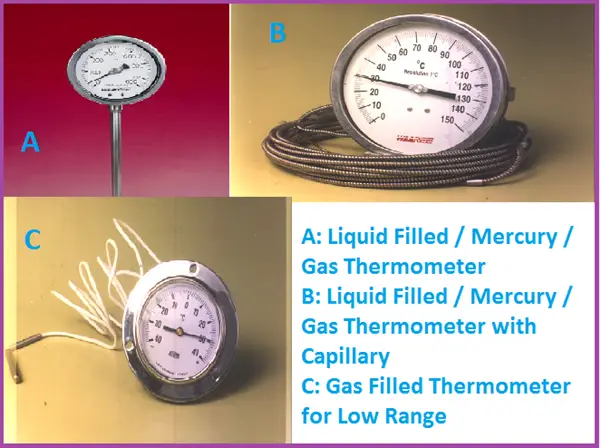
This works on the following principle: Liquid or Gas expands when heated and this change in volume is used for measurement.
A filled thermal system is basically a pressure gauge (generally bourdon type) with a small-bore tubing connected to a bulb acting as a temperature sensor. The complete system is gas-tight and filled with gas or liquid under pressure.
Filled System Selection Criteria
The selection is typically application-oriented.
Ambient temperature compensation.
Scale graduations.
Bulb size and tubing lengths.
Bulb material.
Over-range capacity.
Torque requirements.
Selection of filling fluid/gas.
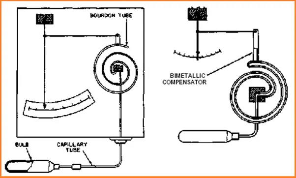
Impact due to Ambient Temperature
Ambient temperature compensation-
Thermal expansion will have a small impact on the reading.
If the range is narrow or the bulb is small and the capillary long then full compensation is required.
Compensation is done either using a bimetallic compensator or by duplicating the spiral and capillary.
A good practice is to have a large bulb diameter.
Fig. 1: Impact due to Ambient Temperature
Liquid filled system
Here the complete system is filled with a liquid (other than mercury) and operates on the principle of liquid expansion.
The filling liquids are – Inert Hydrocarbons like Xylene (C8H10), which has a coefficient of expansion 6 times that of mercury and makes smaller bulbs possible.
The criteria are that the pressure inside the system must be greater than the vapor pressure of the liquid to prevent bubbles of vapor from forming inside the spiral.
Also, the filling liquid should not solidify.
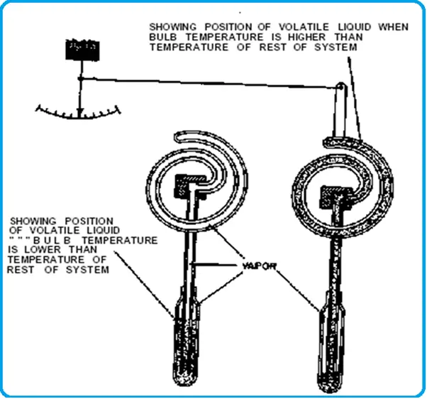
Vapor filled system
Here the filling medium is in both liquid and gaseous form.
The interface between the two must occur in the bulb and this will move slightly with temperature affecting the pressure.
The bulb will be mostly filled with gas while the capillary and spiral would contain liquid.
This is not recommended when the ambient temp. is near to the measured temp.
Fig. 2: Vapor-filled system
Gas-filled system
The operating principle for gas-filled systems is that in a perfect gas confined to a constant volume, the pressure is proportional to the absolute temperature.
Nitrogen is the normal filling media. However, for ranges above 427 Deg. C, this is avoided, as it interacts with steel, which is the bulb material.
For Low temperatures, Helium is used.
Mercury filled system
This is a very common method for measurement.
The response is fast and accurate.
The ambient temperature compensation is less of a problem, as mercury is incompressible.
Fig. 3: Typical images of filled systems
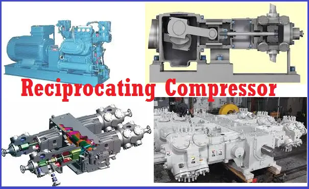
Basics of Reciprocating Compressors / Difference Between Reciprocating Compressor and Rotary Compressor
In a reciprocating compressor, a volume of gas is drawn into a cylinder; it is trapped and compressed by a crankshaft-driven piston and then the high-pressure gas is discharged into the discharge line. It is a positive displacement machine. At any production facility, reciprocating compressors are considered to be one of the most critical and expensive pieces of equipment and hence, require special attention. They are widely used in various industrial facilities to compress gases like:
Air in compressed tool and instrument air systems
Hydrocarbons in the refinery, chemical, and petrochemical plants
Oxygen, Hydrogen, Nitrogen, etc. for chemical processing
Various other gases for storage or transmission
Reciprocating compressors are widely used for compressing dry gases requiring a high compression ratio (discharge pressure/suction pressure).
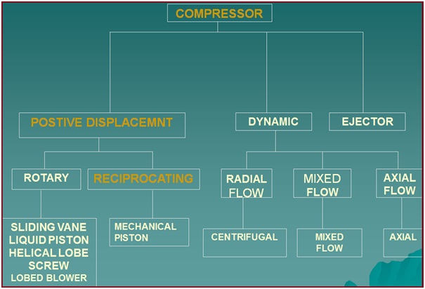
The gas to be compressed enters through the suction manifold and then it flows into the compression cylinder. A piston compresses the gas using a reciprocating motion via a crankshaft. Because of the reciprocating motion of the piston, such compressors are known as reciprocating compressors. The cylinder valves of a reciprocating compressor control the flow of gas through the cylinder; these valves act as check valves. Fig. 1 shows the classification of Compressors.
Fig. 1: Classification of Compressors
Types of Reciprocating Compressors
Depending on the discharge strokes per revolution of the crankshaft, there are two types of reciprocating compressors.
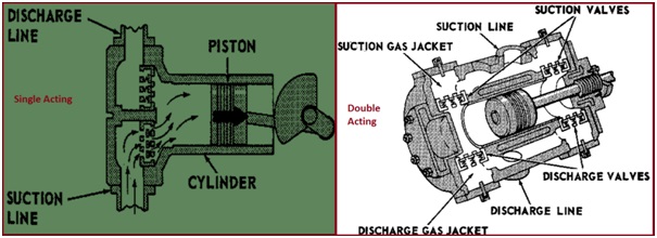
Single – Acting compressor: It is a reciprocating compressor that has one discharge per revolution of the crankshaft. Gas is compressed by only one end of the piston. Contains only one spring-loaded inlet and outlet valve.
Double–Acting Compressor: It is a reciprocating compressor that completes two discharge strokes per revolution of the crankshaft. Gas is compressed by both ends of the piston. Contains inlet and outlet valves at both ends. Most heavy-duty compressors are double-acting.
Fig. 2 Shows the typical configuration of a Single and double-acting reciprocating compressor.
Fig.2: Single and Double acting Reciprocating Compressor
Depending on the drive mechanism of the reciprocating compressor, they are of two types.
Separable Reciprocating Compressor, and
Integral Reciprocating Compressor
The following Table lists down major features of both reciprocating compressor types.
Separable Compressor
Integral Compressor
The compressor and the driver can be separated as driven by separate drives like an electric motor or engine.
Integrally mounted power cylinders drive the compressor and hence can not be separated.
High-Speed Reciprocating Compressors. The typical Operating Speed is 900 -1800 rpm.
Low-Speed reciprocating compressors. The typical operating Speed is 200-600 rpm.
They are normally skid-mounted and the complete skid can be erected at the shop and transported.
Field Erected.
Lower Foundation loads.
Require heavy foundation.
Less vibration severity.
High vibration Severity.
Lower initial Installation Cost.
High Initial Installation cost.
High Maintenance Cost.
Low Maintenance Cost.
Low Efficiency.
High Efficiency.
Separable Compressor vs Integral Compressor
Depending on the number of compression stages before discharge, two types of reciprocating compressors are found:
Single-Stage Reciprocating Compressor, and
Multi-Stage Reciprocating Compressor
The main differences between single-stage and multi-stage reciprocating compressors are listed below
Single-Stage Reciprocating Compressor
Multi-Stage Reciprocating Compressor
Contain Single Cylinder
Contains multiple cylinders
Gas is compressed only once
Gas is compressed multiple times before the final discharge
Lower Compression ratio
Higher Compression ratio
Less Efficiency and Reliability
Improved Efficiency and better reliability
Lower Cost
Higher Cost
Intermittent Operation
Continuous Operation
Single-Stage vs Multi-Stage Reciprocating Compressor
Depending on the speed, Reciprocating compressors are classified as either high speed or slow speed. Typically, high-speed compressors run at a speed of 900 to 1200 rpm, and slow-speed units at speeds of 200 to 600 rpm.
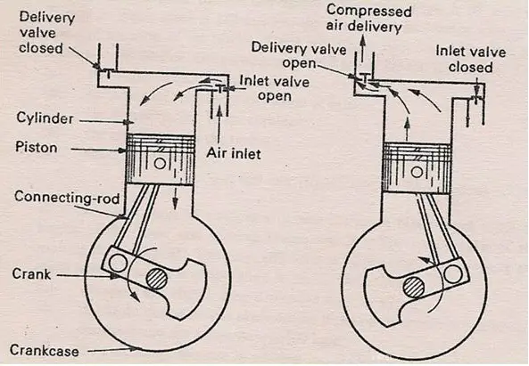
Working of a Reciprocating Compressor
As the name signifies, a reciprocating compressor works by the to and fro motion of the piston inside a cylinder.
When the piston moves downward, it creates a vacuum between the piston top and the cylinder head. This causes the inlet valve to open and low-pressure gas fills in. During this time, inlet valves remain open and discharge valves remain closed.
Next, the piston moves upward forcing the inlet valve to close and the gas is trapped in the cylinder. As the piston moves further the area between the piston head and cylinder reduces which results in gas compression. When the gas pressure exceeds the discharge valve spring resistance, it opens and the gas is transferred to the receiver. The same process is repeated.
Fig. 3: Working Principle of Reciprocating Compressor
Advantages of a Reciprocating Compressor
The main advantages of a reciprocating compressor are:
Broadest pressure range in the compressor family (vacuum to 3000 bar).
Multiple Services on one compressor frame. On a multi-stage frame, each cylinder can be used for separate gas services. For Example, One cylinder is dedicated to propane refrigeration with balance cylinders dedicated to product gas.
Lower capital cost.
Can handle wide variations in capacity with much more ease than any other type.
Complete skid-mounted units allow easy transportation and installation and relocation.
In general, higher efficiencies compared to centrifugal type for the same operating conditions.
Especially suited for low molecular weight applications.
Application limits of Reciprocating Compressors
Reciprocating compressors are limited by the following parameters in their applications:
Flow: they can handle very low flows without significant loss in efficiency.
Capacity: High capacity is limited by cylinder size, stroke length, and speed.
Pressure: Very high pressures up to 3000 bara are practically applied.
Discharge Temperature: Discharge temperature is generally restricted to 135⁰C. For hydrogen-rich services (molecular weight less than or equal to 12) and non-lubricated cylinders, the discharge temperature shall not exceed 120⁰C. Compressed air applications allow higher discharge temperatures
Compression ratio: Typical compression ratios for a single-stage reciprocating compressor are 1.2 to 4.0. The Compression Ratio (Pd/ Ps) is limited by the following;
Maximum Discharge Temperature
Allowable Rod Load
Cylinder Volumetric Efficiency
Horsepower: In gas processing applications power ratings of more than 7.5 MW are rarely found. Special machines with power ratings as high as 30 MW are available for other applications.
Rotating Speed: Low to moderate speeds typically at 300-700 rpm with motors. Moderate to high speeds typically at 600-1800 rpm with motors or gas engines (field gas compression, gas plant, pipeline). Low to moderate speeds in accordance with API STD 618. Moderate to high speeds in accordance with ISO STD 13631.
Codes and Standards for Reciprocating Compressor
Various codes and standards govern the design and manufacture of reciprocating compressors like:
API Standards: API-11P (Packaged Reciprocating Compressors) and API-618 (Reciprocating Compressors for Petroleum, Chemical, and Gas Industry Services)
ISO Standards: ISO-13707 and ISO-13631
Shell DEP: DEP 31.29.40.31
API RP 688 for Pulsation and Vibration Control.
Construction of Reciprocating Compressors
The construction of Reciprocating compressors can be divided into two main areas:
Gas end.
Power end.
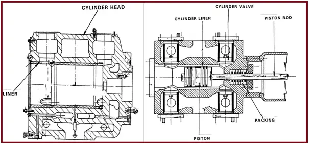
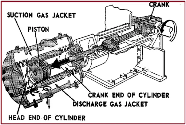
Gas End Parts of a Reciprocating Compressor
The main gas end Parts of the reciprocating compressor (Fig. 4) are
Cylinder
Head
Piston & piston rod.
Suction valves.
Discharge valves.
Piston rod Packing
Suction and discharge gas jacket
Fig. 4: Parts of the reciprocating compressor
Cylinder & Liner
The piston reciprocates inside a cylinder of the reciprocating compressor. To provide for reduced reconditioning cost, the cylinder may be fitted with a liner or sleeve. A cylinder or liner usually wears at the points where the piston rings rub against it. Because of the weight of the piston, wear is usually greater at the bottom of a horizontal cylinder.
Head
The ends of the cylinder are equipped with removable heads, these heads may contain water/liquid jackets for cooling. One end is called the head-end head and the other crank-end head. The crank-end contains packing (a set of metallic packing rings) to prevent gas leakage around the piston rod.
Piston
The piston moves forward and backward to suck and compress the gas. It pushes the gas in the discharge pipe during the compression stroke.
For low-speed (up to 330 rpm) and medium-speed reciprocating compressors (330-600 rpm), pistons are usually made of cast iron.
Up to 7” diameter cast iron pistons are made of solid bars. Those of more than 7” diameters are usually hollow (to reduce cost).
Carbon pistons are sometimes used for compressing oxygen and other gases that must be kept free of lubricant.
Clearance in Piston and Cylinder
As the reciprocating compressor reaches operating temperature, the piston and rod expand more than the liner/cylinder does. In order to prevent seizure adequate clearance should be provided. Similarly, end clearance is also important.
A cold piston is usually installed with one-third of its end clearance on the crank end and two-thirds of its end clearance on the head end.
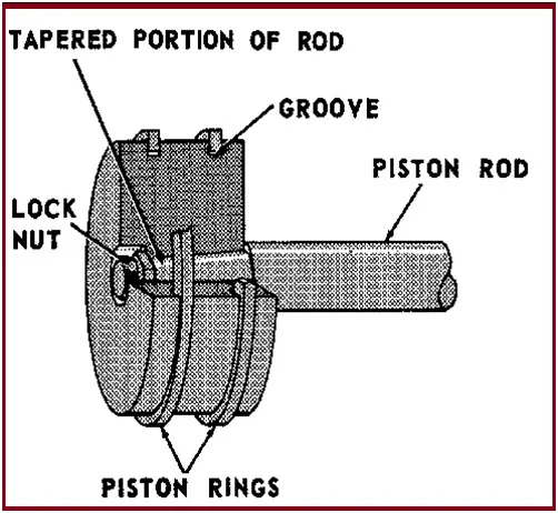
Piston Rings (Fig. 5)
Piston rings provide a seal that prevents or minimizes leakage through the piston and cylinder liner. Metal piston rings are made either in one piece, with a gap, or in several segments. Gaps in the rings allow them to move out or expand as the compressor reaches operating temperature. Rings of the heavy piston are sometimes given bronze, Babbitt, or Teflon expanders or riders. Lubrication is a must for metallic rings. Teflon rings with Teflon rider bands are sometimes used to support the piston when the gas does not permit the use of a lubricant.
Fig. 5: Typical configuration of piston rings
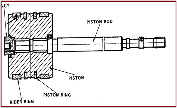
Piston Rod and Piston (Fig. 6)
The piston rod is fastened to the piston by means of a special nut that is prevented from unscrewing. The surface of the rod has a suitable degree of finish designed to minimize wear on the sealing areas as much as possible. The piston is provided with grooves for piston rings and rider rings.
Fig. 6: Typical configuration of Piston Rod and Piston
Piston rod packing
Piston rod packing ensures the sealing of the compressed gas. The piston rod packing consists of a series of cups each containing several seal rings side by side. The rings are built of multiple sectors, held together by a spring installed in the groove running around the outside of the ring.
The entire set of cups is held in place by stud bolts. Inside channels are there for cooling, gas recovery, and lubrication of the piston rod packing.
Oil Seal
An arrangement of scraper rings serves to keep the oil, entrained by the piston rod, from leaking out of the crankcase. The oil scraped is returned to the crankcase reservoir.
Valves
Valves (Suction and Discharge valves): allow gas to enter into the piston during the suction stroke and allow gas to go out into the discharge line during the compression stroke.
There are normally three types of valves, which are
Plate valve.
Channel valve.
Poppet valve.
Power End of a Reciprocating Compressor
Parts of reciprocating compressors that assist in transferring power and converting rotary motion into reciprocating motion are grouped in this category.
Crank Case
The crankcase (Fig. 7) supports the crankshaft. All bearing supports are bored under setup conditions to ensure perfect alignment. The crankcase is provided with easily removable covers on the top for inspection and maintenance. The bottom of the crankcase serves as the oil reservoir. The main pump for lubrication of the crank mechanism is placed on the shield mounted on the side opposite the coupling and is driven by the reciprocating compressor.
Fig. 7: Typical configuration of Crank Case
Crankshaft
Crankshaft receives the power from the Driver and transfers it to the piston. The crankshaft is built in a single piece. On the inside of the shaft are holes for the passage and distribution of lube oil.
Main Bearings
The main bearings are built in two halves, made of steel, with an inner coating of antifriction metal.
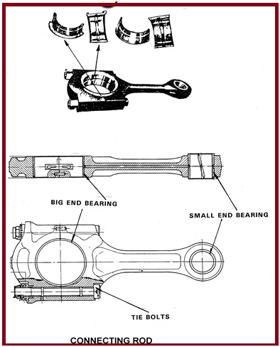
Connecting Rods
Connecting rod (Fig. 8) connect the crankshaft with the piston rod.
The connecting rod has two bearings. The big end bearing is built in two halves. It is made of metal with an inner coating of antifriction metal. The connecting rod’s small end bearing is built of steel, with an inner coating of antifriction metal. A hole runs through the connecting rod for its entire length, to allow passage of oil from the big end to the small end bush.
Fig. 8: Typical configuration of Connecting Rod
Crosshead
Crosshead fastens the piston rod to the connecting rod. The sliding surfaces of crossheads are coated with antifriction metal like Babbit shoe. That permits it to slide back and forth within the crosshead guides. The shoes have channels for the distribution of lube oil. The lubrication is obtained under pressure; it comes out from the two guides of the crosshead slide body.
The connection between connecting rod and crosshead is realized by means of a gudgeon pin. The piston rod is connected to the crosshead by a nut.
Distance piece
The distance piece is used to separate the Gas end and Power End of the Reciprocating compressor.
API 618 defines 4 types of distance pieces for a reciprocating compressor which can be used based on the criticality of service.
Type A – Short single compartment (Where oil carryover to piston packing is acceptable)
Type B – Long Single Compartment (Where oil carryover to piston packing is not acceptable)
Type C – Long-long two-compartment (For critical services like Oxygen and Hydrogen)
Type D – Long-short two-compartment (For Process gas services)
The distance piece is provided with a drain and vent arrangement and if required continuously purge with buffer gas.
Pulsation Dampeners /Bottles for Reciprocating Compressors
Pulsation bottles are provided at suction and discharge to the reciprocating compressor, to keep the pulsation within the desired limit.
A pulsation study was carried out to decide the minimum volume of pulsation bottles.
Lubrication of Reciprocating Compressors
Lubricants reduce friction and therefore wear between moving reciprocating compressor parts. The lubricant also serves as a coolant. Fig. 9 shows a typical Lubrication System.
Fig. 9: Typical Lubrication System
Generally, two types of systems are used to lubricate the positive displacement compressors.
SPLASH SYSTEM
FORCED FEED LUBRICATION
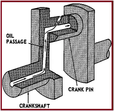
Splash System
It is used in older machines. The level is maintained in the crankcase. Oil is splashed up by the rotation of the crank and the counterweight into the collecting ring. Centrifugal force throws the oil outward through an oil passage to the crank pin.
Forced FEED Lubrication
A pump is used to feed the oil. Oil is pumped under pressure to the required parts. The following are the main parts of the system
Reciprocating Compressor Capacity Control Method
By Recirculation
By VSD
By Valve Un-loader
By Volume clearance pocket
Reciprocating Compressor vs Rotary Compressor
The main differences between a reciprocating compressor and a rotary compressor are tabulated below: