A Vibration Analyzer is a tool to measure, store, diagnose, and analyze the vibration produced by systems or machinery. They work using FFT-based tools that display the magnitude of the vibration and how it varies over the frequency. The main of vibration analyzers is to identify and predict faults and fix them by finding the origin of that vibration.
Vibration analyzers can be used to inspect manufacturing plants, product development labs, building sites, and other places. For the preventative maintenance of manufacturing equipment, a vibration analyzer analyses vibration. The machine’s axis of rotation is also evaluated using a vibration analyzer. If the rotor is out of balance, it can be replaced during the machine’s scheduled downtime.
Vibration analyzer measurements usually detect vibration acceleration, velocity, and displacement characteristics. Vibration is accurately captured in this manner. Vibration measurements may be taken effectively and simply in the field using portable vibration analyzers, which provide precision and mobility. Many vibration analyzers have a memory for saving vibration data for later examination.
For the on-the-job professional, the vibration analyzer is an indispensable instrument. Regardless of the technological issue, each vibration analyzer can complete the tough duty. A sound pressure level meter can also evaluate acoustic vibration (to analyze vibration frequency). It’s possible to detect critical frequencies that can cause harm or create distracting noise levels.
Working Principle of Vibration Analyzers
The working principle of the vibration analyzer is almost identical to the voltmeter; the only variation is measured. The method begins with the sensor or magnetic base device placed on the object whose vibration will be detected. The sensor will instantly give a voltage signal in response to the object’s vibration, which will be relayed over the cable into the vibration analyzer’s transmitter. Take it easy, though, because the numbers indicated on the vibration meter are vibration values in the form of acceleration and velocity, not voltage (speed per unit time). So, given how this vibration meter works, hand-arm and body vibration have two effects.
The operator must choose an appropriate accelerometer based on the mechanical type. Low-frequency accelerometers monitor low acceleration levels and are therefore extremely sensitive. Simultaneously, high-frequency accelerometers record high acceleration levels and are compact with limited sensitivity.
The piezoelectric accelerometer is typically used to measure vibrations with a frequency greater than one hertz (Hz). It features a high-frequency feature to measure vibrations in the higher frequency range. They are mostly utilized in industrial operations for automated installation vibration monitoring and diagnostic tests.
Uses of Vibration Analyzer
The application of a vibration analyzer is multi-fold. Some of the common uses of vibration analyzers are listed below:
- A vibration analyzer can measure the vibration of structures such as buildings, motorways and bridges, railway tracks, airport quarries, and other major industrial facilities.
- The vibration occurs in this building due to natural events such as wind, weather, and earthquakes, or interior components such as the elevator, ventilation, and HVAC systems. As a result, vibration testing aids in identifying building regions that are more susceptible to vibration.
- A vibration analyzer is also used to determine how much the human body vibrates.
- The instrument’s metrics include vibration acceleration, velocity, and displacement.
Features of a Vibration Analyzer
The following are the important elements to consider when purchasing a vibration analyzer:
1. Make sure the number of input channels is accurate:
Vibration analyzers come in various configurations, with the most common being two to four input channels. Recording two channels simultaneously is generally sufficient for balancing, phase analysis, Bode graph, and ODS functions. On the other hand, using triaxial accelerometers and balancing two planes necessitates the usage of four channels.
2. Frequency Range:
The frequency range of a vibration analyzer is defined by two factors: the analyzer’s highest sample rate and the accelerometer’s maximum frequency range. A system’s Sample Rate is the number of measurements it can make in one second. As a result, the device’s maximum frequency will be half of its sampling rate.
3. Lines of resolution:
The number of resolution lines determines how many points will be used to integrate the spectrum. Although the actual name is “Points,” the term “Lines” is still used, most likely since it was coined for audio FFTs that were plotted with bars (or lines). The resolution of a spectrum is sometimes mistakenly equated with the lines of resolution; however, this is not valid. Because the LR does not distinguish between a large or small frequency range, a lower frequency range with the same number of lines will show better resolution than a higher range with the same number of lines.
4. Check for additional functions:
The features of analyzers are most likely the part that varies the most from one analyzer to the next.
i) FFT: The heart of an analyzer is the spectrum, which is required by practically all analysis functions. Rectangular, Hamming, and flattops are FFT measurement tools and Windows functions.
ii) Parameters of measurement: Acceleration, Velocity, Displacement, and the Envelope of Acceleration (Demodulation or equivalent, useful for early bearing fault detection)
iii) Vibration Data Collector: A decent vibration analyzer should also be able to capture vibration data. At the very least, it should have a method for storing and organizing machine recordings to keep track of their history and trends. This is an important issue to consider because you will be dealing with this part of the system daily. It’s critical to have an intuitive and simple database interface to avoid wasting time later.
iv) Waveform of Time: This chart is created by vibration analyzers as the sensor receives the signal. Although it is rarely used, some auxiliary functions, such as Circular Time Wave Form, can be beneficial in detecting patterns in gearboxes or bearings.
v) Bearing database: Bearing vibration analysis identifies fault frequencies related to bearing geometry; hence this function is critical. As a result, you’ll have access to a comprehensive bearings database, as well as manufacturer information for fault estimates.
vi) Sensor used: The vibration’s acceleration is proportional to the output voltage. Because they incorporate small amplifiers and filters to remove noise, most sensors require power. Accelerometers are often used in vibration analyzers because of their wide frequency and amplitude ranges of animal noise. In exchange, they translate acceleration into other vibration-related metrics like velocity and displacement.
vii) Probes that measure displacement: The output signal is proportional to the vibration displacement. They are typically non-contact sensors, making them excellent for sensing shaft vibrations and eccentricity. It is advantageous if the vibration analyzer you select allows you to attach various types of sensors. There are some machines for which an accelerometer is not the best tool. Oil bearings are an example because oil dampens vibrations, making inaccurate accelerometer measurements.
5. Requirement for other features like
- Cloud connectivity requirements,
- Technical support needs,
- Portability characteristics,
- Power requirements, etc.
Handheld Vibration Analyzer
A handheld vibration analyzer is a mobile phone-sized gadget with a larger screen and spectrum display and is well-prepared for route-taking. They are lightweight and convenient to use. Due to the slow CPUs in these vibration analyzers, the number of lines of resolution, memory, and functionalities is limited, necessitating the use of PC-based software to supplement capabilities.
Features Of Hand-held Vibration Analyzer
- A hand-held vibration analyzer readily measures the vibration levels of bearings, gears, and spindles for maintenance purposes.
- Hand-held vibration analyzer simple enough to use that only a few people need to know how to utilize it.
- An industrial accelerometer, cable assembly, mounting magnet, and headphones for audio monitoring are commonly included.
- A hand-held vibration analyzer is a battery-powered engine that’s small and portable.
- A hand-held vibration analyzer is mostly used to check the severity of fans, motors, and pumps and test the dc bias voltage of accelerometers for troubleshooting installed sensors and connections.
Portable Vibration Analyzer
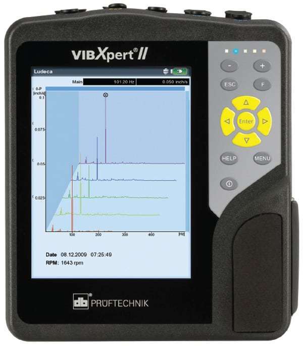
Electrical signal monitoring is a feature of a portable vibration analyzer, that assists in the diagnosis of the condition of rotating machinery. Fig. 1 below shows an example of a typical portable vibration analyzer.
Features of Portable vibration Analyzer:
- The overall vibration data are given in displacement, velocity, and acceleration
- A portable vibration analyzer is usually light in weight and simple to operate.
- A portable vibration analyzer usually has an automatic power-off feature and displays real RMS data.
- A portable vibration analyzer incorporates a back-light display that makes measuring even in dimly lit or enclosed spaces.
- Portable vibration analysis can detect vibrations in machinery produced by out-of-balance, misalignment, gear breakage, bearing failures, and other factors.
Conclusion:
A vibration analyzer is a critical power and energy meter in an electrical power testing system. You may quickly test and quantify vibration values with the help of this instrument, and the findings will be accurate. So, go ahead and start looking for the best vibration analyzer for your service potential starting right now.
Online Vibration Basics Course
Hope, the subject of vibration analyzers is clear to you now. To get a detailed understanding of vibration and related theories you can opt for any of the following online courses with lifetime access:
- Vibration acceptance criteria for rotodynamic pumps- ISO, HI
- Basics of vibrations and vibration measurement
- Vibration measurement and acceptance criteria as per API 610
- Complete Mechanical Vibration Online Course
- Fundamental steps in the study of Mechanical Vibrations
References and Further Studies
- Vibration Analysis Explained | Reliable Plant. (n.d.). Vibration Analysis Explained | Reliable Plant. https://www.reliableplant.com/vibration-analysis-31569.
- Best Vibration Analyzer. (2019, January 24). ERBESSD INSTRUMENTS. https://www.erbessd-instruments.com/articles/best-vibration-analyzer/.
- The Basics Of Vibration Analysis. (2021, October 27). Limble. https://limblecmms.com/blog/vibration-analysis/.
- Vibration Meter: Types, Features & Applications. (2020, August 3). Blog on procurement of all industrial, office supplies | Shake Deal. https://www.shakedeal.com/blog/what-is-a-vibration-meter/.