An emergency shutdown system or ESD system is a highly reliable control system for providing a safety layer during emergency situations. It helps to prevent situations from having catastrophic impacts economically, environmentally, or operationally. Emergency Shutdown Systems in any plant minimize injury to working personnel & the environment or damage to equipment, by protecting against leaks, hydrocarbon escape, fire outbreaks, explosions, etc. The application of emergency shutdown systems has been substantiated in the oilfields (oil wellheads), Nuclear plants, oil and gas processing plants, steam and gas turbine power plants, chemical & petrochemical plants, boilers, geothermal industries, etc. During an emergency situation, the process operations are stopped by the ESD system, therefore, isolating the hazard to escalate.
Functions of an Emergency Shutdown System
All emergency shutdown systems should always work at the back end throughout the plant operation as it is one of the main security systems. The major functions of an emergency shutdown system are:
- Shut down of the system or equipment during a critical situation
- Isolate electrical equipment
- Proper control of ventilation during an emergency
- Stop or isolate hydrocarbon sources from potential hazard situations.
- Blowdown and depressurization.
- Prevent dangerous event escalation like prevention of ignition and explosion.
- To protect personnel, asset, and the environment.
Note that critical situations may be triggered in any plant by various factors but emergency shutdown systems should be able to handle those in an effective manner.
Emergency Shutdown system design considerations
The design of the Emergency Shutdown or ESD system shall take into account the needs resulting from normal operation and shall also fulfill the requirements that may arise during other possible (and likely to occur) abnormal or down-graded configurations. Depending on the type of operating plant and functions, ESD system design will vary.
However, the below-listed issues shall be adequately addressed when relevant:
- Tripping or stopping a unit or equipment does not necessarily eliminate all sources of hazards.
- Due to the loss of essential utilities like air, essential power, hydraulics, etc., new hazards can appear anytime. The emergency shutdown system should be designed to identify and mitigate or alarm regarding the risk of such hazards.
- All operating configurations that the ESD system generates shall be stable, safe, and reversible.
- The ESD system shall be compatible with the re-start philosophy. The inevitable inhibitions of the control and safety systems during the re-start sequence shall be identified and shall be limited in number, time, and duration.
- ESD system design shall provide specific attention to non-routine operating conditions, simultaneous operations, and down-graded situations.
- Particular operating conditions may require a different shutdown logic than that, or the combination of those, applicable under normal circumstances. For example, An installation normally operates under different conditions, e.g. high, medium, or low pressure. Each condition may require a different ESD logic, but the differences shall be limited to process shutdowns. Emergency shutdowns shall result in the same actions independent of the condition. Before switching over between different ESD logics, the proper line-up of equipment and the status of valves need to be verified.
- The Emergency Shutdown system shall be used to continuously monitor the safety parameters of the plant and shall take actions to maintain the safety of the plants on demand.
- The ESD system diagnostics shall show the following minimum fault / healthy state status but not limited to:
- Circuit breakers tripped
- Power feeders healthy
- Fuse Failure
- Power supply removed
- CPU fault
- Battery failure
- Power supply failure
- Communication Failure
- Input/ Output Module failure
- The input/ Output Module removed
- Each channel failure
- Panel internal temperature high
- Others as supplied by the manufacturer.
Working of Emergency Shutdown System
An emergency shutdown system works by monitoring the plant condition using field-mounted sensors, valves, trip relays, and inputs to a control system as alarms. The control system performs a cause-and-effect analysis of the above parameters to determine plant health. The system will minimize the effects in case of abnormal behavior by reducing the number of plant items available or shutting down part of the system. For example, In case of a fire hazard, a Fire Damper control system may override the existing controls to open or close vents as needed, and close fire doors.
Normally, for plants, a shutdown matrix is defined. Three to four shutdown levels based on decreasing criticality are decided and the complete plant is categorized. In the process control system, various safety loops and devices are organized as complementary barriers. For each installation, an ESD/SD logic shall be defined covering all the installations and represented in an ESD/SD logic diagram.
Components of an Emergency Shutdown System
The following components shall be part of an emergency shutdown system:
- Dedicated Process Transmitters
- Shut Down Valves, Normally Fail to Close Type
- Logic Solver
- Blowdown valves
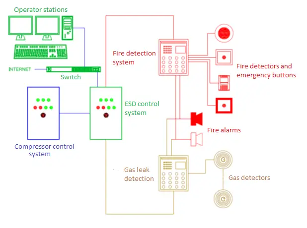
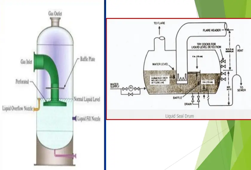
Fig. 1 below shows a Typical Emergency Shutdown System in its basic form.