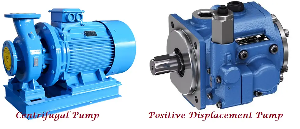
Centrifugal and Positive displacement pumps are the two main categories of pumps used widely. The main purpose of both groups of pumps is to pump fluid from one point to another. But they have some distinct differences. The working principle of both these pump groups is different. A Centrifugal Pump transfers the kinetic energy of the motor to the liquid through the rotating impeller. This increases the velocity and pressure at the discharge. The discharge velocity remains constant when the motor rpm is constant. On the other hand, Positive displacement pumps trap a fixed volume of fluid in their cavity and force it to discharge into the pump outlet. So, it is a constant volume device. Positive displacement comes in rotary, reciprocating, or diaphragm style. Centrifugal pumps are high-capacity and relatively low-head pumps whereas positive displacement pumps are low-capacity high-head pumps. In the next paragraphs, we will discuss, other major differences between Centrifugal and Positive Displacement Pumps.
Centrifugal vs Positive Displacement Pump: Fluid Handling
With an increase in the fluid viscosity, the efficiency of the centrifugal pump decreases due to frictional losses. That’s why centrifugal pumps are not suitable for highly viscous fluids. Whereas, with an increase in viscosity, the efficiency of the positive displacement pump increases.
Also, positive displacement pumps can handle liquids with suspended solids and liquids with abrasive particles.
Centrifugal vs Positive Displacement Pump: Pump Speed & Shearing of Liquid
Centrifugal Pumps are high-speed pumps. It causes shearing of liquids. Hence, not suitable for sensitive mediums. On the other hand, positive displacement pumps operate at lower velocities which causes very little shear.
Centrifugal vs Positive Displacement Pump: Pump Performance
In centrifugal pumps, the flow varies with change in pressure whereas in positive displacement pumps flow remains constant with changing pressure. For both pumps, flow can be regulated by changing the speed. Fig. 1 below shows how a centrifugal pump and a positive displacement pump behave with changes in different factors.
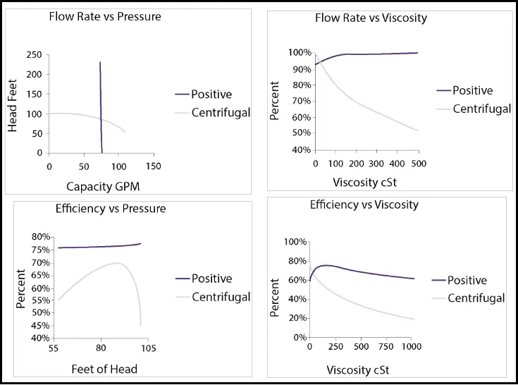
The above curves show that “with an increase in Viscosity, Flow Rate and Efficiency of the centrifugal pump drops to a huge extent. Also, with changes in pressure head centrifugal pump flow rate and efficiency changes”
In a centrifugal pump the Net Positive Suction Head required (NPSHr) varies as a function of flow determined by pressure. But in a Positive Displacement pump, the NPSHr varies as a function of flow determined by speed. The lower the speed of a Positive Displacement pump, the lower the NPSHr.
Centrifugal vs Positive Displacement Pump: Efficiency
Centrifugal pumps perform better in the center of the curve known as BEP (best efficiency point). At lower or higher pressure levels, the centrifugal pump efficiency reduces. It is therefore suggested to operate centrifugal pumps within a window of 80-110% of its BEP for optimum pump performance. When moving far enough to the right or left from the curve center, pump life is reduced due to shaft deflection or increased cavitation.
Positive displacement pumps can operate at any point of the curve. The efficiency increases with an increase in pressure.
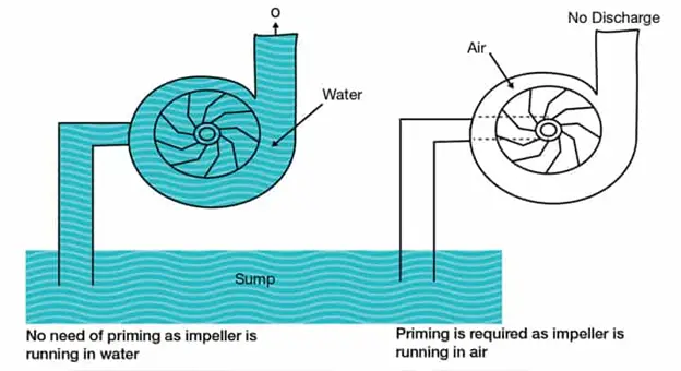
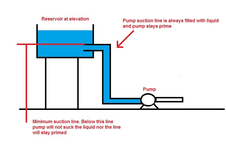
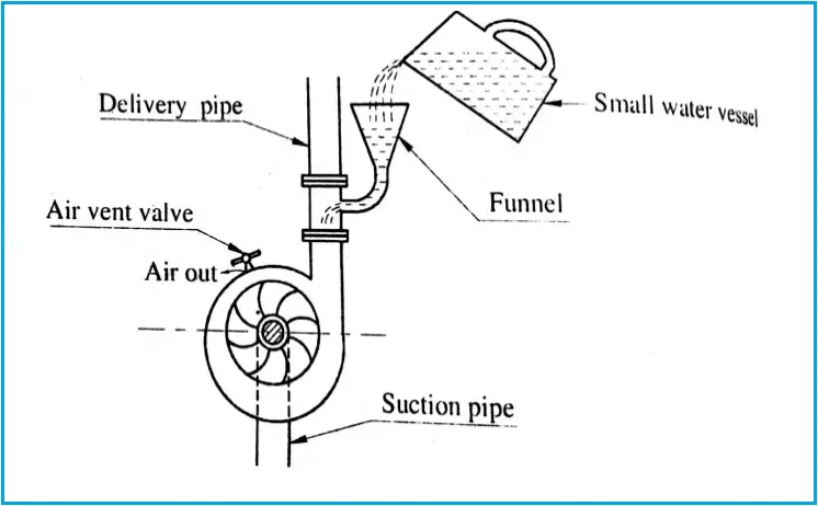
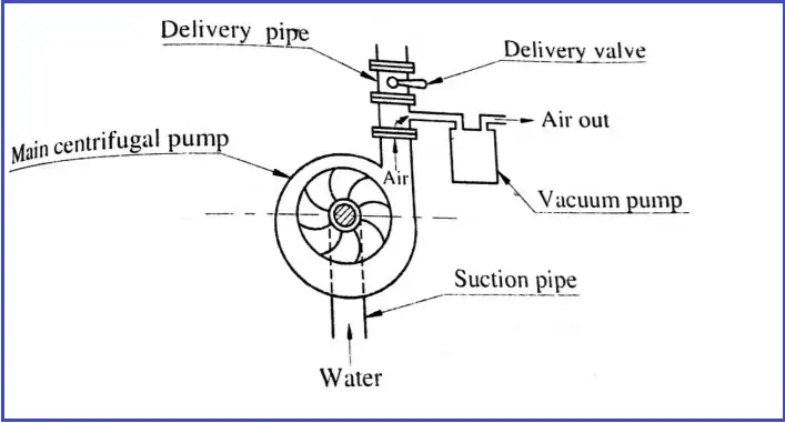
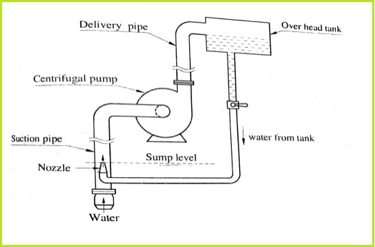
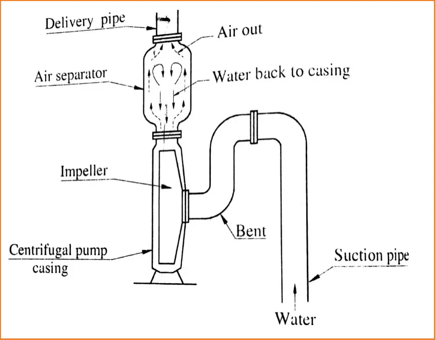
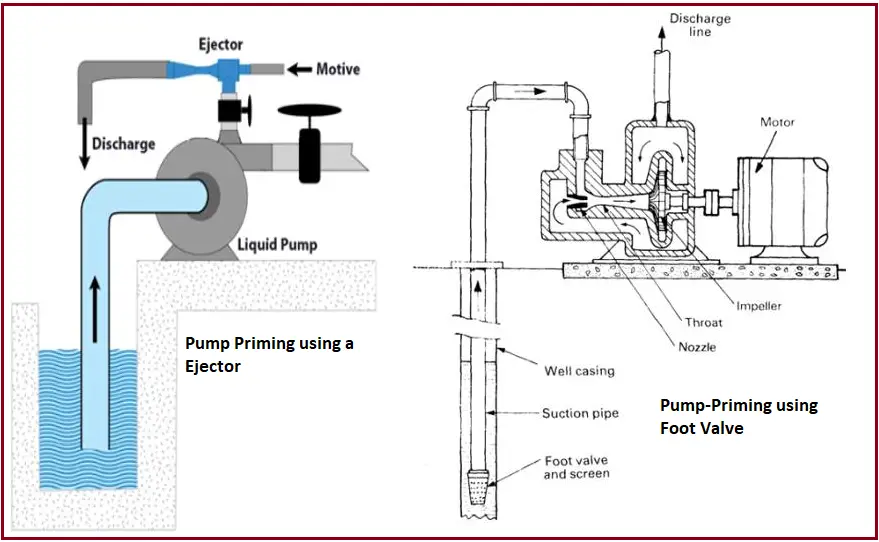
Centrifugal vs Positive Displacement Pump: Priming Requirement
Standard centrifugal pumps require priming before starting the pump. Whereas positive displacement pumps create a vacuum on the suction side; So fluid can automatically enter the pump. Positive displacement pumps are called self-primed pumps.
Centrifugal vs Positive Displacement Pump: Cavitation
Due to the presence of entrapped gases, centrifugal pumps are more susceptible to cavitation as compared to positive displacement pumps. Also, during low-flow operation, centrifugal pumps are more prone to overheating.
Centrifugal vs Positive Displacement Pump: Series and parallel operation
In parallel operation of two or more pumps to increase the flow. Normally, positive displacement (PD) pumps in parallel will provide larger flows as compared to centrifugal pumps as PD pumps will inherently compensate for the higher system pressure, and in the case of centrifugal pumps due to frictional losses the combined flow is not doubled.
For series operations in centrifugal pumps, the head created by each pump is added. But for PD pumps in series operation, no advantage is obtained and hence, PD pumps are not run in series.
Centrifugal vs Positive Displacement Pump: Which one to Select?
A Positive Displacement pump will be a preferred selection in the following situations:
- For high viscous applications.
- For variable pressure conditions.
- When the pump will be operating away from the BEP.
- For changing viscosity conditions.
- For very high-pressure applications.
- For shear-sensitive liquids.
However, these are only a few criteria. Actual pump selection is more detailed and an experimental study is required for selecting the right pump.
Centrifugal vs Positive Displacement Pump: Cost
The operational and maintenance cost of a positive displacement pump is normally lower than the a centrifugal pump. The initial cost can be more or equivalent to a centrifugal pump depending on the positive displacement pump type.
Due to Low-speed operation, Positive displacement pump seals work longer as compared to centrifugal pump seals.
Centrifugal vs Positive Displacement Pump: Applications
Centrifugal pumps are best suited for thin liquids possessing low viscosity levels like water, thin oils and fuels, and chemicals. It is, therefore, the most commonly used for high-volume applications with high flow rates at low pressures. Some of the popular applications of centrifugal pumps include
- Irrigation
- Municipal water and water supply systems
- Chemical, Petrochemical, and light fuel transfer stations
- Air conditioners and water circulators
- Boiler feeds
- Firefighting
- Cooling towers
On the contrary, positive displacement pumps are used for high pressure and low flow conditions to move highly viscous fluids. Some of the popular applications include
- Manufacturing facilities to move thick paste and jelly.
- Municipal Sewage systems.
- Thick Oil Processing
- Food Processing plants
The main differences between Centrifugal Pump and Positive Displacement Pumps are tabulated below
| Centrifugal Pump | Positive Displacement Pump |
| The efficiency of centrifugal pumps decreases with increasing viscosity | The efficiency of the positive displacement pump increases with increasing viscosity |
| The flow of the centrifugal pump varies with changing pressure | The flow for positive displacement pumps is insensitive to changing pressure |
| The Pump Efficiency decreases at both higher and lower pressures for centrifugal pumps. | The efficiency of positive displacement pumps increases with increasing pressure |
| For centrifugal pumps, Priming is Required | Pump Priming is not required for positive displacement pumps. |
| Centrifugal pumps provide a Constant Flow | Positive displacement pumps provide a Pulsating Flow |
| Centrifugal pumps are High-Velocity Pumps | Positive displacement pumps have Low internal velocity |
| Centrifugal pumps are High Capacity and Low Head | Low Capacity and High Head is the characteristic of positive displacement pumps. |
| Centrifugal pumps work based on Centrifugal Action | Positive displacement pumps work based on rotary, reciprocating, or diaphragm principle |