In the field of fluid mechanics, understanding the behavior of fluids in motion is of utmost importance. One crucial parameter that helps characterize the flow regime is the Reynolds number. Named after the pioneering scientist Osborne Reynolds, this dimensionless number provides insight into the transition between laminar and turbulent flow. In this article, we will delve into the concept of the Reynolds number, its equation, significance, and how it influences fluid flow.
What is Reynold’s Number? Definition of Reynold’s Number
Reynolds Number is a very important quantity for studying fluid flow patterns. It is a dimensionless parameter and is widely used in fluid mechanics. Reynolds Number of a flowing fluid is defined as the ratio of inertia force to the viscous force of that fluid and it quantifies the relative importance of these two types of forces for given flow conditions.
The concept of Reynold’s number was introduced by George Stokes in 1851. However, the name “Reynolds Number” was given with the name of the British physicist Osborne Reynolds, who popularized its use in 1883. The Reynolds number depends on the relative internal movement due to different fluid velocities. For fluid flow analysis, Reynold’s number is considered to be a prerequisite.
Importance of Reynolds Number
Reynolds Number (Re) is a convenient parameter that helps in predicting if a fluid flow condition will be laminar or turbulent. We know that Reynolds Number (Re)=inertia force/viscous force.
When viscous force dominates over the inertia force, the flow is smooth and at low velocities; the Reynolds Number value is comparatively less and the flow is known as laminar flow. On the other hand, when inertia force is dominant, the value of the Reynolds number is comparatively higher and the fluid flows faster at higher velocities and the flow is called turbulent flow. At low Reynolds Number Values (Re<2100) the viscous force is sufficient enough to keep fluid particles in line making the flow laminar which is characterized by smooth and constant fluid motion. While at large Reynold Number values (Re>4000), the flow tends to produce chaotic eddies, vortices, and other flow instabilities making the flow turbulent. With an increase in Reynolds Number the turbulence tendency of the flow increases.
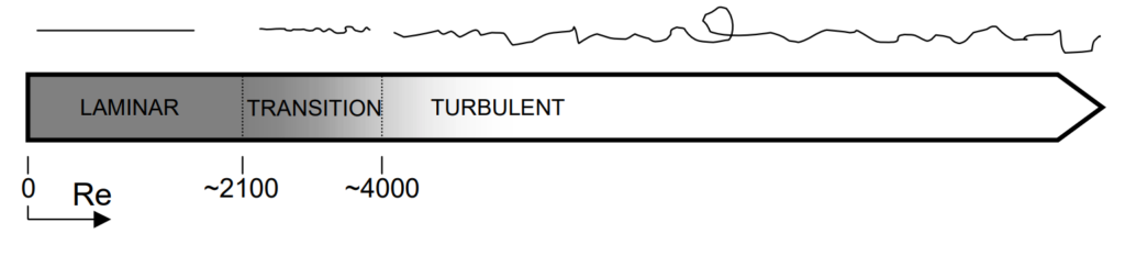
“2100<Reynolds Number (Re)<4000” indicates a flow transition from laminar to turbulent and the flow consists of a mixed behavior. However, note that the value of Reynolds number (Re) at which turbulent flow begins is dependent on the geometry of the fluid flow, which is different for pipe flow and external flow.
The Reynolds number associated with the laminar-turbulent transition is known as the Critical Reynolds Number. This laminar to turbulent transition is a highly complicated process, which is not yet fully understood.
The Equation for Reynolds Number
Mathematically, The Equation for the Reynolds number is represented as
Re=ρuD/μ
where
- ρ is the fluid density Kg/m3)
- D is a length scale that characterizes the scale of the flow motions of interest (m)
- u is the fluid velocity (m/s)
- μ is the fluid dynamic viscosity (Pa.s or N.s/m2 or kg/m.s)
- the term μ/ρ is known as kinematic viscosity, ν (m2/s)
Hence the formula for Reynold’s number can be written as Re=ρuD/μ=uD/ν
The Reynolds number (Re) of a flowing fluid can easily be calculated by multiplying the velocity of fluid flow by the pipe’s internal diameter and then dividing the result by the kinematic viscosity of the fluid.
Components of Reynolds Number Formula
Let’s understand the components of the Reynolds Number Formula:
Inertial Forces: Inertial forces arise from the tendency of a fluid to resist changes in its state of motion. They depend on the density of the fluid (ρ) and the velocity of the fluid (u). A higher density or higher velocity will result in greater inertial forces.
Viscous Forces: Viscous forces, on the other hand, are the internal frictional forces between adjacent fluid layers that resist the flow. These forces depend on the dynamic viscosity (μ) of the fluid. A higher viscosity implies stronger viscous forces.
Characteristic Length (D): The characteristic length (D) represents a characteristic dimension of the object or the flow domain. It could be the diameter of a pipe, the chord length of an airfoil, or any other relevant length scale. The choice of characteristic length is crucial and depends on the specific flow situation.
Unit of Reynold’s Number
Let’s find the dimension of Reynold’s number. The Primary dimension of ρ is (M/L3) and the velocity is (L/T)
Again the primary dimension of diameter/length is L and viscosity μ is (M/LT).
Substituting all these values in the above-mentioned formula of Reynold’s number we get [{M/L3 * L/T * L}/ (M/LT)]=M*L*L*L*T/L3*T*M=MTL3/MTL3=1 Which means Reynolds Number is dimensionless or unitless. The same concept can be put forth as follows:
As the Reynolds Number is the ratio of two forces, there is no unit of Reynolds Number. So, Reynold’s Number is dimensionless.
Factors Affecting Reynolds Number
The main factors that govern the value of the Reynolds Number are:
- The fluid flow geometry
- Flow velocity; with an increase in flow velocity the Reynolds number increases.
- Characteristic Dimension; with an increase in characteristic dimension the Reynolds number increases.
- Fluid Density; with a decrease in fluid density the Reynolds number value decreases.
- Viscosity; with an increase in viscosity the value of the Reynolds number decreases.
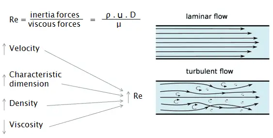
So, in one sentence we can conclude that Reynolds Number is directly proportional to Flow Velocity, Characteristic Dimension, and Fluid Density while inversely proportional to fluid viscosity.
Applications of Reynold’s Number
The Reynolds number plays a crucial role in fluid mechanics and has significant practical implications. Here are a few areas where the Reynolds number finds applications:
Flow Analysis and Design:
Understanding the Reynolds number is vital in the analysis and design of fluid flow systems. It helps engineers and scientists predict the behavior of fluids in pipes, channels, and around objects. By knowing the flow regime, appropriate design considerations can be made to optimize efficiency and minimize pressure losses.
Drag and Lift Forces:
The Reynolds number influences the drag and lift forces acting on objects moving through a fluid. In the case of aerodynamics, for instance, the Reynolds number determines the flow regime around an aircraft wing or an automobile, affecting factors such as lift, drag, and overall performance.
Heat Transfer:
The Reynolds number has implications for heat transfer processes. It helps in determining the convective heat transfer coefficient, which is crucial in applications such as cooling systems, heat exchangers, and thermal management.
Fluid Mixing:
The Reynolds number is a valuable parameter in understanding and controlling fluid mixing processes. It helps determine the efficiency and effectiveness of mixing operations in various industries, including chemical engineering, pharmaceuticals, and food processing.
Other Applications:
As Reynolds number is used for predicting laminar and turbulent flow, it is widely used as a design parameter for hydraulic and aerodynamic equipment. The Reynolds number for laminar flow is less than 2100. The value of the Reynolds number is a significant necessity for fluid flow analysis.
For the design of piping systems, aircraft wings, pumping systems, scaling of fluid dynamic problems, etc Reynolds number serves as an important design tool. To simulate the movement of any object in any fluid, the Reynolds Number is required.
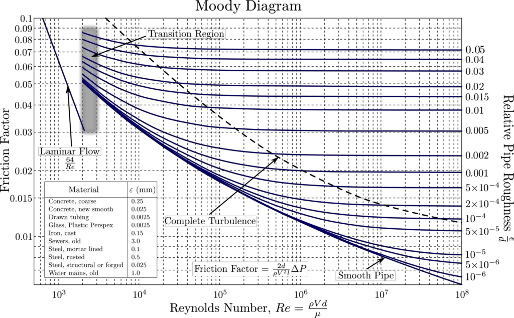
Reynold’s number is used to calculate the value of the drag coefficient. In the calculation of pressure drop and frictional losses, the Reynolds number plays an important role. The following diagram (Fig. 3), known as the Moody chart provides a correlation between friction factor, Reynold’s Number, and Relative roughness and is widely used in solving fluid flow problems.
Reynold’s number (Re) is also used to calculate the value of friction factor (f) using the Colebrook Equation as mentioned below:
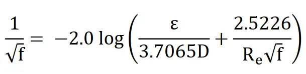
In the above equation, ε=Absolute Roughness.
Reynolds Number Values
The following table provides some typical Reynold Number values
| Sr No | Item | Typical Reynolds Number |
| 1 | Laminar Flow | <2100 |
| 2 | Turbulent Flow | >4000 |
| 3 | Person Swimming | 4 × 10⁶ |
| 4 | Blue Whale | 4 × 10⁸ |
| 5 | Smallest fish | 1 |
| 6 | Atmospheric tropical cyclone | 1 x 10¹² |
| 7 | Bacterium | 1 × 10⁻⁴ |
| 8 | Blood flow in the brain | 1 × 10² |
| 9 | Blood flow in the aorta | 1 × 10³ |
| 10 | Fastest fish | 1 × 10⁸ |
Reynolds Number for Laminar Flow
Laminar flow is the smooth flow in layers. There is little or no mixing and the fluid velocity is typically lower. The motion of the fluid particles is ordered without any cross currents. This is typically found in fluids of high viscosity and at lower velocities. The value of Reynold’s Number for Laminar flow is less than 2100.
Reynolds Number for Turbulent Flow
In turbulent flow, there is turbulence and unpredictable mixing. The velocity is high and fluids do not move in layers similar to laminar flow. Waves in the sea or river, storms, etc are examples of typical turbulent flow. The Reynolds Number for Turbulent flow is usually considered greater than 4000.
Critical Reynolds Number
The transition from laminar to turbulent flow is not abrupt but gradual. There is a critical Reynolds number, known as the critical Reynolds number, below which the flow remains laminar and above which it becomes turbulent. The specific value of the critical Reynolds number depends on various factors such as the geometry of the object, surface roughness, and fluid properties.
Low and High Reynolds Number
At low values of Reynolds Number Re<<1, the inertial effect becomes negligible. The flow behavior is dependent on the viscosity and the flow is stable. Whereas when the Reynolds Number Re is very very high, the viscous effects are negligible. The fluid flow behavior depends on the momentum of the fluid and the flow is unsteady.
Conclusions
The Reynolds number provides valuable insight into the flow regime of fluids and the transition from laminar to turbulent flow. By considering the interplay between inertial and viscous forces, engineers and scientists can better predict and analyze fluid behavior in various systems. Understanding the Reynolds number is essential for optimizing design, predicting performance, and ensuring efficient and safe operation of fluid systems across numerous fields of application.