As Pipe Stress Engineers, we all, in some way or other, have handled the assignment of modeling and analyzing parallel lines routed over pipe racks or sleepers. Often these lines require Expansion Loops to have sufficient flexibility. However, although may be routed kilometers, these lines often do not have any interconnection between them. Therefore, normal practice is to model these lines in separate ‘.C2’ files and carry out stress analysis and expansion loops sizing and positioning separately. Now, suppose if we could model all lines running parallel to each other in a corridor and with the same design code (e.g. B31.3) in a single ‘.C2’ file, then not only we could view and review all the lines together, but also we could size and locate expansion loops for each line with respect to the others. This would not only reduce the modeling and analysis efforts but would also enable us to handle a lesser number of CAESAR II native files.
This is pretty well possible with the help of the ‘Block Operation’ and ‘Coordinate’ features in CAESAR II. In my earlier post titled “ADVANTAGE OF USING ‘BLOCK OPERATION’ IN CAESAR II, “ I tried to explain ‘Block Operation’. In this post, I would attempt to highlight the effective use of the ‘Coordinate’ feature.
Let us take the case of two lines running parallel to each other over a Pipe Rack, and supported in the same locations.
Parameters for Line 1:
Design Code = ASME B31.3
MOC = ASTM A106 Gr. B
Size = 12”
Sch. = STD
Corrosion Allowance = 1.5 mm
Design Pressure = 1200 kPa(g)
Design Temperature = 175OC
Fluid Density = 900 kg/m3
Insulation = Mineral Wool
Insulation Thickness = 50 mm
Cladding Thickness = 0.7 mm
Cladding Density (Aluminium) = 2700 kg/m3
Parameters for Line 2:
Design Code = ASME B31.3
MOC = ASTM A106 Gr. B
Size = 10”
Sch. = STD
Corrosion Allowance = 1.5 mm
Design Pressure = 1800 kPa(g)
Design Temperature = 150OC
Fluid Density = 900 kg/m3
Insulation = Mineral Wool
Insulation Thickness = 50 mm
Cladding Thickness = 0.7 mm
Cladding Density (Aluminium) = 2700 kg/m3
Let us assume these two lines are having a gap of 500 mm between centerlines.
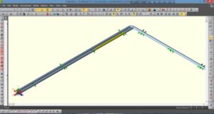
First, we model Line 1 as per the given parameters.
Fig. 1: Modeling of line 1
Line 1 starts at Node 10 and ends at Node 370.
Now, we invoke ‘List Input’.
Fig. 2: Invoking List Input in Caesar II
Then, at the ‘List Input’ window, we select all elements, right-click, select ‘Block Operation’ and then select ‘Duplicate’.
Fig. 3: Duplicating Elements in Caesar II
In the ‘Block Duplicate’ window, under the ‘Options’ tab, we select ‘Identical’, under the ‘Insert Copied Block’ tab, we select ‘At End of Input’, and input ‘400’ in the ‘Node Increment’ box, and click ‘OK’.
Figure – 4
Now, we input ‘500’ in the box of X coordinate in ‘Enter Global Coordinates (mm.) for Node 410’ under the ‘Global Coordinates’ window.
Figure – 5
Now, we have created the geometry of Line 2, but still with the parameters of Line 1. So, we change the parameters as applicable.
Figure – 6
Figure – 7
Then, we close the ‘List Input’ window.
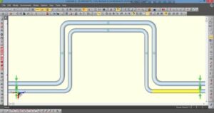
Now, we are ready with two lines that are running in the same route, supported at the same locations, but still requiring some manual modifications at the elbows of Line 2.
Figure – 8
So, we reduce the lengths of elements before and after the first elbow by 500 mm. Likewise, we adjust the expansion loop of Line 2 to arrive at the following geometry in Figure – 9.
Figure – 9
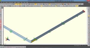
Finally, we increase the lengths of elements before and after the last elbow by 500 mm.
Figure – 10
This completes the parametric and geometric adjustments of Line 2.
Now, both of the lines are ready for onward analysis.
Note: Although this is a useful and smart way of working, the stress analyst must use his/her judgment for use of this feature, particularly if the lines are to be analyzed under different codes, it is recommended not to use this feature. Also, the model shown as an example is a very simplified one. An analyst may encounter more complex problems, and the extent of manual adjustment is likely to vary from little to more on a case-by-case basis.
Telegram Channels / Telegram Groups for Piping and Related Engineering
Telegram Application, the best Whatsapp alternative has gained tremendous traction in just a couple of years since its launch. In February 2016, the app maker stated that the number of active monthly users surpassed the 100 million mark, adding 350,000 users each day who send 15 billion messages per day.
Advantages of Engineering Telegram Groups and Telegram Channels
In recent times, due to WhatsApp’s limitation of only 257 members, engineers and designers from EPC organizations found telegram channels and telegram groups as one of the best methods of communication, discussion, knowledge sharing, job sharing and clarifying doubts between the group and channel members. As there is no limitation of the number of members similar to WhatsApp these telegram groups become very popular. In this article, links to join a few such top engineering telegram channels and top engineering telegram groups will be provided for the readers to take benefit.
Background of Piping and Related Engineering Telegram Channels and Telegram Groups
Maximum of these telegram groups and channels were started in 2015, and these are one of the most popular groups to get correct answers to the question in different fields from industry-experienced persons. Even though the Basic language in these groups is Persian, still members are aware of the English language. Hence, anyone can use his queries in the English language and he will get answers in English.
Free Kids Worksheets Telegram Channel: Join this telegram channel for free educational worksheets for your kids from Kindergarten to Class IV (Grade 4). Link to join the group is: https://t.me/practiceworksheets
Learning Process: Process Engineering telegram Group for friendly discussion of process engineering problems among group members. Link to join this group is: https://t.me/joinchat/EdebRAvpWwbqdcNhX9016g
To join any of the above-mentioned groups or channels install telegram apps in your mobile from google play store or iPhone store. After installing open the apps and register your mobile no similar to WhatsApp. Once registered, search the above groups or channels in the telegram app and the group will appear. Otherwise, click the above links on your mobile after opening the telegram app. Click on join and start following the activities of the group. Readers are requested to list down other telegram groups in the comments section to help others.
Stress Analysis of Pump Piping (Centrifugal) System using Caesar II
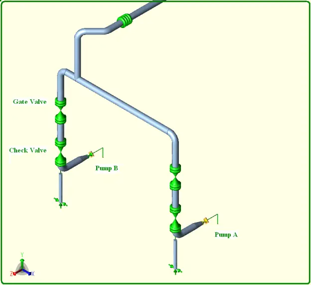
Every power or process piping industry uses several pumps in each unit. The analysis of pump-connected piping systems is considered very critical. In this article, I will try to elaborate on the method followed for the stress analysis of a centrifugal pump piping system. The stress system consists of typical discharge lines of two centrifugal pumps (Pump A and Pump B). Fluid from these two pumps is pumped into a heat exchanger. As per P&ID, only one pump will operate at a time, other pumps will be a stand-by pump. I will explain the stress analysis methodology in three parts:
Fig. 1: Sample pump piping model as it looks in Caesar II
Modeling of Pump in Caesar II
For modeling the pump we require a vendor general arrangement drawing or outline drawing. All rotary equipment is modeled as a weightless rigid body in Caesar II. From the outline drawing, we need to take the dimensions to some fixed point. Let us take the example of the outline drawing shown in figure 2.
Fig. 2: Sample outline drawing for a centrifugal pump
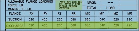
From the above drawing, we can get the dimensions for elements 10-5000 as 8.5 inches and elements 5000-5020 as 6.19 inches. At node 5020 we will provide a fixed anchor. During the modeling of the above elements, we need to use line size and thickness as the diameter and thickness of the equipment. Line temperature and pressures as equipment properties. We have to provide an anchor (with a C-Node) at node 10 for checking nozzle loads which we will compare with the allowable value as provided in Fig. 3 below:
Fig. 3: Allowable nozzle load values as mentioned in Equipment GA drawing
In absence of allowable load value, the Pump design code (API 610 for API pumps, ANSI HI 9.6.2 for non-API pumps) can be followed for the same.
After the pump is modeled as a rigid body the piping modeling need to be done from pump-piping interconnection flanges.
Preparation of Analysis Load Cases
Along with normal load cases, two additional load cases need to be prepared. Normally in the refinery and petrochemical industry, one pump operates and the other pump acts as a stand-by pump. So we have prepared load cases as follows:
1. Hydrostatic case (WW+HP HYD)
2. Operating case with both pumps operating (W+T1+P1 OPE)
3. Operating case with the total system in maximum design temperature ( W+T2+P1 OPE)
4. Operating case with pump A operating and pump B Stand by (W+T3+P1 OPE)
5. Operating case with pump B operating and pump A Stand by (W+T4+P1 OPE)
6. Operating case with the total system in minimum design temperature ( W+T5+P1 OPE)
Next all normal load cases like static seismic, static wind, etc are to be built as per stress analysis or flexibility specification.
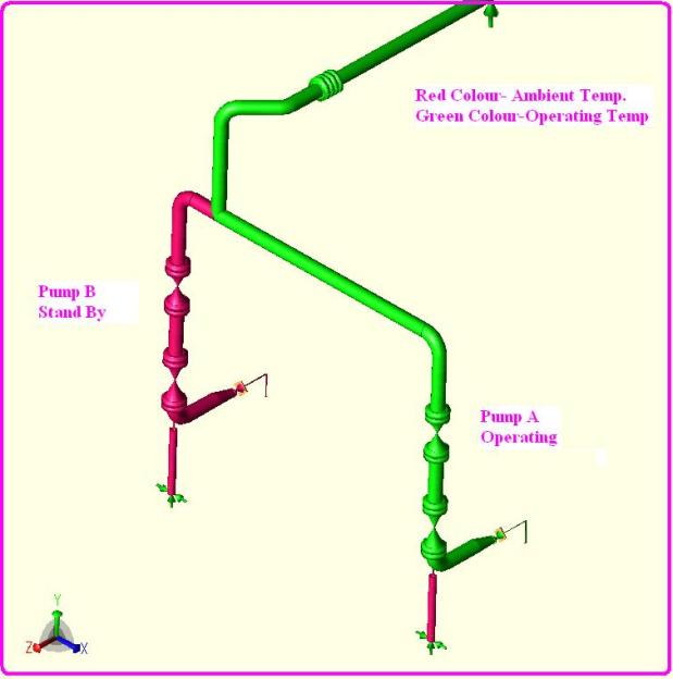
When pump A is in operating condition and pump B stand by, the normal pipe operating temperature has to be inserted till the Tee connection for pump A and ambient temperature will be the input for pump B as shown in Fig. 4. Similarly, reverse the input when pump B is operating.
Fig. 4: Operating-Stand By Temperature profile for a two-pump system
After the equipment is modeled completely start modeling the piping following dimensions from piping isometric drawings. Try to make a closed system. Normally pump lines are connected to some vessel, tank, or heat exchangers. So it will create a closed system. Then run the analysis to check stresses, displacements, and loads.
Analyzing the output Result
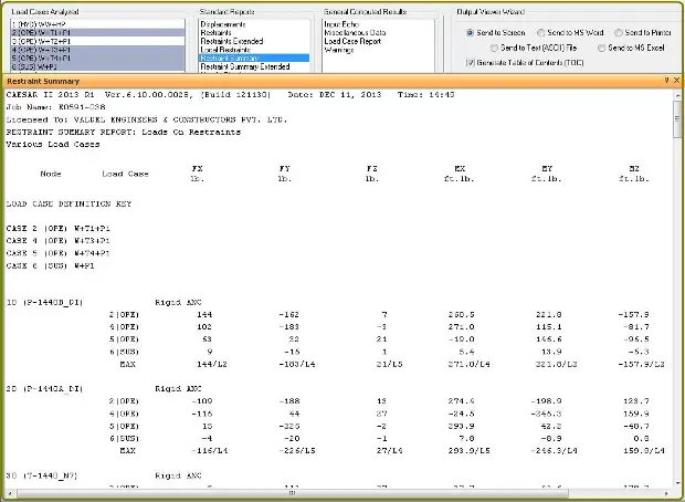
Once Caesar completes its iteration process we can see the output results in the output window. At nozzles (the nodes which we anchored with a CNode) we can check the force values. These values we have to compare these with the allowable values. If the actual values are less than the allowable values then the nozzle is safe. Otherwise, we have the make changes in supporting or routing to bring the nozzle load values within allowable. A sample output restraint is provided in Fig. 5 for your reference.
Fig 5. Typical output results for a two-pump system
As can be seen from the above figure we are checking nozzle loads in load cases 2, 4, 5, and 6. For rotary equipment, normally nozzle qualification in design or upset temperature is not required.
Always remember to provide the first piping support from the pump nozzle as adjustable support (or a spring hanger support) to aid in alignment.
In the case of 3 pump systems, normally two pumps will be operating and one pump will be stand by. So input and prepare load cases accordingly. If you have any confusion or want to add more please write in the comments section.
Video Tutorial for Pump Piping Stress Analysis
The following video explains the pump piping stress analysis methodology for 3 pumps in detail.
From last few months few of the readers are asking to provide some guidelines for stress analysis of Plastic Piping System. This video tutorial by Mr. Alex Matveev (Developer of PASS/START-PROF Software) will explain the steps for stress analysis of plastic i.e, PVC, PP, PB, PVDF and HDPE piping using PASS/Start-Prof Software(Widely used stress analysis software in Russia-Used since 1965). Hope it will be useful for all piping engineers.
The article will cover the following points in several parts:
How to create a simple plastic piping model in START-PROF software and run the analysis.
Stress Analysis Theory for analyzing plastic piping systems following Codes/Standards.
How the plastic piping system works.
In part 1 of this article one simple plastic piping system is modeled and its analysis methodology is shown.
New construction of piping systems requires some type of cleaning of debris or contaminants. Debris can be defined as substances such as dirt, grease, construction materials such as wood, wire, hard hats, tools, weld slag, rust and scale, and any other small objects that could be misplaced inside the diameter of piping systems. Proper cleaning of Piping Systems is required dependent upon service requirements.
Piping System Cleaning Requirements
All piping systems shall be flushed with water. Water flush is accomplished through the hydro-testing of piping systems. If the water being drained still has evidence of debris, continue to flush with water until no evidence of debris exists.
Lines that require cleaning should be identified on the Mechanical Flow Diagrams. The Process Engineering Group (Process Department) shall set the limits based on the service requirements and equipment being protected from debris and contaminants generated during construction.
Certain process services require chemical cleaning of Piping Systems. The process engineer shall be responsible for identifying services that require chemical cleaning. Typical examples of services requiring chemical cleaning are listed below:
Super High-Pressure Boiler Feed Water and High-Pressure Steam
Product Shipping Lines
Specialty Chemical /Catalyst lines
Oxygen
Hydrogen Peroxide
The designer should be responsible for verifying all steps to remove debris that would be detrimental to the process fluid, including the provision of any temporary facilities for carrying out the chemical cleaning procedures.
The cleaning method used should be selected based on the facilities available. Steam and detergent cleaning is much less costly than acid or mechanical cleaning. Each project specification must indicate the type of contamination/debris to be removed.
All systems shall be sealed after cleaning to keep out dirt and moisture. Cleaning in place with chemical cleaning solutions shall be compatible with all components of the piping system; otherwise, components that would be adversely affected by the cleaning solution shall be temporarily removed.
The use and disposal of cleaning solutions must be in accordance with plant policy or local regulations (or both).
Mechanical Cleaning: Rotating shafts, brushes, compressed air, and flying grit are hazards. Use protective equipment dictated by the site.
Chemical Cleaning: Acids and other chemicals, heated solutions, steam pressure hoses, spills, and sprays are hazards. Provide protective clothing, eye protection, safety showers, and facilities to neutralize spills of spent chemicals. Personnel should not breathe ferroxyl solution (or other chemicals) vapors that may be harmful. Adequate respiration must be provided when testing or cleaning in enclosed areas with inadequate ventilation.
Vapor Cleaning: Steam, condensate, and other hazards are associated with chemical cleaning. Controlled discharge of vapors to the atmosphere or condensate cooled by water sprays is essential to minimize personal contact.
Pipe Cleaning procedures
Procedure for Water Flush:
Flush the pipe with chloride-free clean water.
Thoroughly drain the pipe and dry it if required. Drying can be done by wiping or by blowing with clean, dry compressed air or inert gas.
Procedure for Air Blow:
Blow with clean, dry compressed air. Use a sufficient volume of air to create high velocity in the pipe.
Procedure for Steam and Detergent Cleaning:
Steam-clean with a water solution of Pennwalt Corp. Cleaner MC-79, Oakite Products, Inc. Oakite 33, or approved equal. (Mix 1 gal MC-79 with 9 gals clean water; mix 1 gal Oakite 33 with 6 gals clean water.)
Drainpipe thoroughly and flush with clean water.
Dry the pipe by wiping or by blowing with clean, dry compressed air or inert gas.
Procedure for acid Cleaning for Stainless Steel:
The choice of acid cleaning solution depends upon the composition, heat treatment, and form of the stainless steel to be cleaned. Choose the acid-cleaning solution as follows:
For mill products or castings in the solution-annealed condition of Type 300 or 400 series and Carpenter 20 Cb (UNS N08020), Alloy B (UNS N10001), or Alloy C-276 (UNS N10276) material, or to weldments, mill products, or castings of CF-8, CF-8M, CF-3, CF-3M, and SW20M (CN-7M): use a nitric-hydrofluoric acid.
For weldments of Type 304, 316, or any of the other non-extra low carbon (ELC), non-stabilized grades, or for severely sensitized items (such as those that have been stress-relieved) of any of the grades (including ELC and stabilized): use a weak acid.
Procedure for Pickle (Sulfuric Acid method) for Carbon Steel:
Pickle with a solution of one part Metclean No. 1 or equivalent (inhibited sulfuric acid) 3 to 10 parts of clean water. Heat and maintain the pickling bath between 71 and 82 °C (160 and 180 °F).
Pump the solution through the pipe or immerse the pipe in a pickling tank until clean.
Flush with clean water.
Inspect and repeat steps 2 and 3 if necessary.
Rinse with a neutralizer solution.
Dry as required by the process in which the pipe is being used.
Procedure for Pickle (Citric Acid Method) for Carbon Steel:
Pickle in a solution of 3-1/2 gal of water per lb of citric acid (required anhydrous granular citric acid). Heat and maintain pickling solution between 82 and 88 °C (180 and 190 °F).
Pump the solution through the pipe or immerse the pipe in a pickling tank until clean.
Flush with clean water.
Inspect and repeat steps 2 and 3 if necessary.
Rinse with a neutralizer solution of 5.0 percent soda ash (Na2CO3).
Flush with rust inhibitor consisting of 0.5 percent sodium nitrite (NaNO2), 0.25 percent disodium phosphate (Na2HPO4), and 0.25 percent monosodium phosphate (NaH2PO4).
Dry as required by the process in which the pipe is being used.
Procedure for Mechanical Cleaning for Stainless Steel:
Blast-clean inside of pipe and fittings with clean, iron-free sand or alundum grit. Repeat if free iron is found. Use ferroxyl test if required. Blast-cleaning of clad material should not be carried to the point of seriously reducing the cladding thickness.
Walnut-shell blast provides very smooth interior surfaces. Blast inside of pipe and fittings until desired results are obtained.
For brush cleaning, use stainless steel wire
Note: Anyone, or all, of the mechanical cleaning procedures, may be required to effectively clean stainless steel pipe and fittings when weld spatter or scale (or both) have formed from welding.
Procedure for Mechanical Cleaning for Carbon Steel:
Blast clean inside of pipe and fittings. Wire brushing with power rotary wire brushes is an alternate method. A rotary cutter followed by wire brushing should be used on heavily rusted, pitted, and weld-spattered pipe, and on the pipe with a tightly adhered scale.
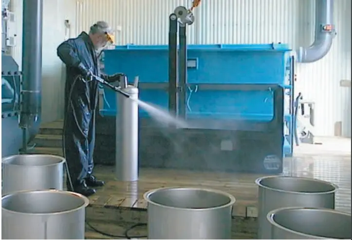
Pipeline pigging is the process of using a specialized device called a “pig” to clean, inspect, and maintain pipelines used for transporting liquids or gases. Pigs are typically made of various materials, such as rubber, urethane, or steel, and are inserted into the pipeline through access points called “pig launchers” and “pig receivers.”
The pig is propelled through the pipeline using the fluid flow, and its design allows it to remove debris, sediment, or other buildups from the pipeline’s interior walls. This cleaning process helps to prevent corrosion, improve flow rates, and maintain the integrity of the pipeline.
In addition to cleaning, pipeline pigging can also be used to inspect pipelines for damage or defects, such as cracks, corrosion, or leaks. Specialized inspection pigs can be equipped with sensors and cameras that allow for the detection and identification of these issues, helping to prevent potential leaks or failures.
Pipeline pigging can be performed on a regular maintenance schedule, or as needed when issues are suspected. The use of pigs can help reduce downtime and maintenance costs, as well as improve the overall safety and efficiency of the pipeline. However, it is important to ensure that pigging operations are conducted safely and that all necessary precautions are taken to prevent accidents or damage to the pipeline.
The process of driving the pig through a pipeline by the fluid is called a pipeline pigging operation. The term pig was originally referred to as Go-Devil scrapers which were driven through the pipeline by the flowing fluid trailing spring-loaded rakes for removing the wax off the internal walls. People believe that “PIG” is the short form of the term “Pipeline Inspection Gauge”. During pipeline pigging a squealing noise that sounds like a pig squealing arises, hence the name “PIG” is given.
Pipeline Pigging is used to perform various cleaning, clearing, dimensioning, maintenance, inspection, process, and pipeline testing operations on new and existing pipelines. A pipeline-pigging system includes
Pigs.
Pig Launcher.
Pig Receiver.
Reasons for Pipeline Pigging
A pipeline Pigging operation is performed to
Maintain a reliable and acceptable performance of the pipeline in terms of safety and product delivery at an economical cost.
Provide a defined margin of safety for operating the pipeline at its designated pressure.
Provide timely information on all pipeline defects such that repairs can be carried out according to a managed schedule.
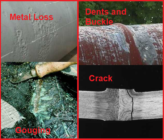
There are several kinds of flaws and defects in pipelines that can lead to pipeline failure, the main families being:-
Metal loss
Cracks or crack-like defects
Laminations and other mid-wall defects
Geometric anomalies
There are
basically three reasons to pig a pipeline:
To separate dissimilar products.
To remove undesirable materials.
To perform internal cleaning, inspections, and maintenance.
Working of the Pipeline Pigging Process
Pipeline Pigs are inserted into a Pig Launcher and then the pressurized flow is applied to the rear of the device. The flow forces the pig to move into the pipeline. The force applied by a pig when it moves in a pipeline can be estimated by multiplying the cross-sectional area of the back of the pig by the pressure applied to the rear of the pig.
In General, the outside diameter of most pigs will be sized to be larger than the internal bore. This size difference creates a resultant ‘interference’ that enables the pig to scrape and remove debris as it moves through the pipeline. The type of pig employed determines the degree of effectiveness in cleaning a pipeline. Various other factors like flow rate, pig speed, length of the pipeline, number of pigging runs, pressure, temperature, the volume of debris to be removed, number and type of bends, pipeline elevations, pigging frequency, etc are also to be considered.
When the pig reaches the other end of the pipeline it is captured in a Pig Receiver which is isolated via a shut-off valve, allowing the pig to be safely removed.
Which Pipelines are ‘Piggable’?
Most of the pipelines constructed of materials like Carbon Steel, Stainless Steel, Duplex Stainless Steel, AC, GRP, HDPE, DICL, Cast Iron, Plastic, PVC, and others can all be pigged. Additional considerations for piggable pipelines are:
The decision to pig any pipeline is considered by a thorough analysis of the line in conjunction with field-proven experience and advice offered by a reputable pigging specialist.
Pipeline Pig Types
Three categories of pigs are used to accomplish the above-mentioned tasks. They are:
Utility Pigs, are used to perform functions such as cleaning, separating, or dewatering.
In-Line Inspection Pigs: They provide information on the line condition along with the extent and location of any problems.
Gel Pigs are used in conjunction with conventional pigs to optimize pipeline dewatering, cleaning, and drying tasks.
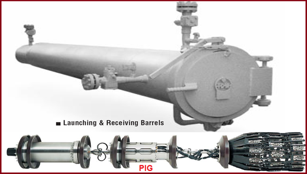
Fig. 1: PIG, Launching & Receiving Barrel
Utility PIGs
Based on the fundamental purpose, Utility pigs can be divided into two groups as listed below:
Cleaning pigs
Remove solid deposits.
Remove Semi-solid deposits.
Remove Debris.
Sealing pigs
Provide an interface between
two dissimilar products.
Provide a good seal in order to
sweep liquids.
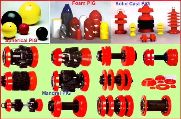
Types or forms of Utility pigs:
Spherical Pigs (inflatable,
solid, foam, and soluble).
Foam Pigs (Polly-Pigs).
Mandrel Pigs
Solid Cast Pigs.
Spherical PIGs (Fig. 2):
There are four basic types of spheres:
inflatable.
Solid.
Foam.
Soluble.
Spherical PIGs are normally used for
Removing liquids from wet gas systems.
Serving to prove fluid meters.
Controlling paraffin in crude oil pipelines.
Flooding pipeline to conduct hydrostatic tests.
Dewatering after pipeline rehabilitation or after new construction.
They should never
be run in lines that do not have special flow tees installed.
Foam PIGs (Fig. 2):
They are normally manufactured in a bullet shape.
Coated pigs may have a spiral coating of polyurethane, various brush materials, or silicon carbide coating.
The standard dimension of foam pig length is twice the diameter.
Foam pigs are lightweight, compressible, expandable, and flexible.
They have the ability to travel through multiple diameter pipelines and go around mitered bends and short radius 90o bends.
They also go through valves with as little as a 65% opening.
Foam pigs are that they are a one-time-use product.
High concentrations of some acids will shorten life.
Foam pigs are inexpensive.
Foam pigs are used for pipelines for
proving,
drying
wiping,
removal of thick soft deposits,
condensate removal in wet gas pipelines,
pigging multiple diameters
scraping and mild abrasion of the pipeline.
the shorter length of runs,
Mandrel PIGs (Fig. 2):
The mandrel pig can be used for
cleaning pig,
sealing pig,
combination of both.
The seals and brushes can be
replaced to make the pig reusable.
These pigs are designed for
long runs.
The cost of redressing the pig
is high, and larger pigs require special handling equipment to load and unload
the pig.
Occasionally the wire brush
bristles break off and get into instrumentation and other unwanted places.
Smaller-size mandrel pigs do not negotiate 1.5D bends.
Fig. 2: Various types of PIGs
Solid cast PIGs (Fig. 2):
Solid cast pigs are usually molded in one piece.
The materials used for the preparation of solid cast Pig are neoprene, nitrile, Viton, and polyurethane).
Solid cast pigs are considered sealing pigs although some solid cast pigs are available with wraparound brushes and can be used for cleaning purposes.
The solid cast pig is available in the cup, disc, or a combination cup/ disc design.
Because of the cost to redress a mandrel pig, many companies use the solid cast pig up to 14 inches or 16 inches.
Solid cast pigs are used
In removing liquids from product pipelines.
removing condensate and water from wet gas systems.
Controlling paraffin build-up in crude oil systems.
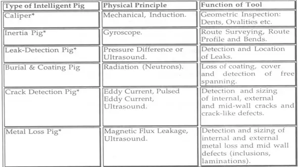
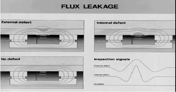
Inline Inspection PIGs
In-line inspection PIG tools are used to carry out various types of tasks including:
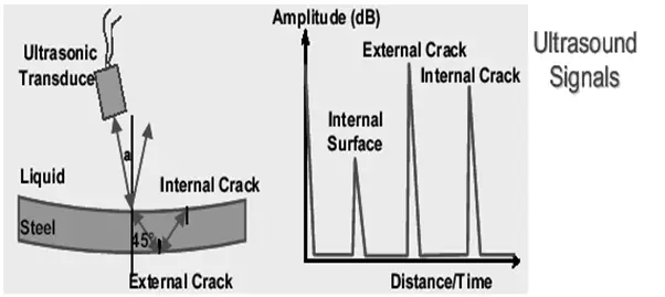
They work in a pulse-echo mode with a rather high repetition frequency.
Straight incidence of the ultrasonic pulses is used to measure the wall thickness and 45º incidence is used for the detection of cracks.
Working principle of Ultrasonic Inline inspection Pig (Fig. 6):
Fig. 6: Ultrasonic inline inspection
GEL PIGs
Types of Gel Pigs
High-viscosity sealing gels
Commissioning cleaning gel
systems
Polymer Gel Pig
Debris pickup gel.
Batching or separator gel.
Hydrocarbon gel.
Dehydrating gel.
The Principal
Pipeline applications for gel pigs are as follows:
Product separation.
Debris removal.
Line filling/ hydro testing.
Dewatering and drying.
Condensate removal from gas lines.
Inhibitor and biocide laydown.
Special chemical treatment.
Removal of stuck pigs.
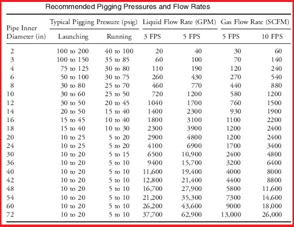
Pipeline Pigging Pressure
The following table gives the recommended pipeline pigging pressures and flow rates for pipeline pigging operations.
Fig. 7: Recommended Pipeline Pigging Pressure
Applications of Pipeline Pigging
During pipeline construction, pigging is used for debris removal, gauging, cleaning, flooding, and dewatering.
During fluid production operations, pigging is utilized for removing wax in oil pipelines and removing liquids in gas pipelines.
pigging is widely employed for pipeline inspection purposes such as wall thickness measurement and detection of spanning and burial.
Pigging is also run for coating the inside surface of the pipeline with inhibitors and providing pressure resistance during other pipeline maintenance operations.
In recent times, Smart PIG is used to travel through a pipeline which gathers important pipeline data like the presence and location of corrosion or other irregularities on the inner walls of the pipe. That’s why the pipeline pigging using smart pigs are often termed as Intelligent Pigging.
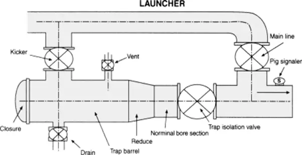
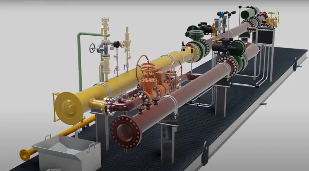
What is a PIG Launcher?
Fig. 8: Pig Launcher
A Pig Launcher is a device, generally, a Y-shaped funnel section of a pipeline system from where the PIG is launched. It is basically a pressurized container that can be opened to insert the PIG. Refer to Fig. 8 and Fig. 9 for a clear idea of what a Pig Launcher looks like.
Fig. 9: Typical Pipeline Pig Launcher
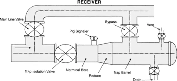
What is a PIG Receiver?
Fig. 10: Pig Receiver
A pig receiver is a container or device to receive a pipeline pig out of the pipeline without interrupting the flow. This forms a part of the pipeline pigging system. Both pig launchers and receivers are known as pig trap assemblies.
Both the Pig launcher and receiver constitute the following components:
Pipeline pigging products refer to the various types of pigs and related equipment used in pipeline pigging operations. These products include both cleaning and inspection pigs, as well as the launchers, receivers, and other tools used in the pigging process.
Cleaning pigs are used to remove debris, sediment, and other buildups from the interior walls of pipelines. These pigs can be made of various materials, including rubber, polyurethane, or steel, and can be designed with different shapes and sizes to accommodate different pipeline diameters and cleaning requirements.
Inspection pigs are used to detect and identify issues such as cracks, corrosion, or leaks in pipelines. These pigs are typically equipped with sensors, cameras, or other specialized equipment that can provide detailed information about the condition of the pipeline.
Launchers and receivers are used to insert and remove pigs from the pipeline. These are typically large, heavy-duty vessels designed to withstand the high pressures and temperatures present in pipelines.
Other pipeline-pigging products may include various tools and accessories, such as brushes, scrapers, and gauges, that can be used to clean or inspect pipelines.
The selection of pipeline-pigging products will depend on the specific requirements of the pipeline and the pigging operation. Working with a qualified pigging equipment supplier or engineer can help ensure that the appropriate products are selected for the specific application and that they meet all necessary safety and performance standards.
Pipeline Pigging Companies
There are many renowned pipeline-pigging companies around the world that offer a range of pigging products and services. Here are a few examples:
Baker Hughes: A multinational oilfield services company that offers a range of pigging products and services, including pigging tools, cleaning and inspection pigs, and data analysis software.
T.D. Williamson: A global pipeline services company that offers a range of pigging products and services, including pigging tools, inspection pigs, and pipeline cleaning services.
ROSEN Group: A leading provider of inspection, integrity, and maintenance services for the energy industry, including pipeline pigging products and services.
Pigs Unlimited International: A leading supplier of pipeline pigging products, including cleaning and inspection pigs, launchers, receivers, and other pigging equipment.
NDT Global: A provider of advanced pipeline inspection and integrity services, including high-resolution geometry and mapping tools and inspection pigs.
Quest Integrity: A global provider of advanced inspection and engineering services, including pipeline pigging products and services.
Pigtek Ltd: A UK-based manufacturer and supplier of pipeline pigging products and services, including cleaning and inspection pigs, launchers, receivers, and other pigging equipment.
Conclusions:
Pigging is a vital tool that helps to achieve Pipeline integrity by providing
Safety and product delivery at an economical cost.