As piping constitutes a major chunk of any refinery, chemical, petrochemical, or power generating industries there is always a need of purchasing various piping and mechanical items. There must be an approved procurement procedure for the smooth functioning of this process and receiving items in the construction site without much delay. In this article, We will explore the major Steps involved during the Procurement/Purchase Process of piping/mechanical items for the Oil and Gas Industry.
Many types of equipment and items need to be purchased in the piping project from different vendors/suppliers. Before finalization of the vendor/ supplier to get the pipe material, there are many phases/ steps which need to be followed as mentioned below:
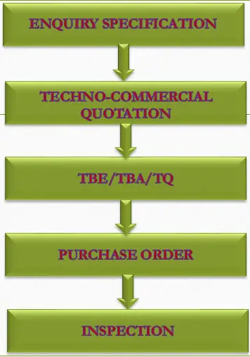
In the first step, an inquiry specification (normally specifications specifies all technical requirements, preliminary drawings, quality requirements, etc.) for the required equipment/item is floated to several different vendors to get a techno-commercial quotation. Normally each company has a list of approved vendors. The inquiry is generally sent to the approved vendors/ suppliers. In case the item is not available with the approved vendors then other vendors are requested to go through the approval procedure and they are included in the approved vendor list.
Based on the specification mentioned in the purchase requisition (PR) Vendors prepare an offer and send it. After receiving offers from the different vendors/suppliers, each offer is checked and evaluated from a technical viewpoint first and then a cost point. If there are any changes/deviations or if there are points that the vendor has not confirmed, it has to be clarified through technical queries/TQ. This process may take a few days to complete.
After receiving the replies to all the technical queries and the deviation request from the suppliers the originating engineer will decide if the vendor is technically suitable for that particular inquiry. He may select several vendors as suitable based on technical and qualitative requirements.
The specification engineer then populates the replies of all the vendors/suppliers in a common document (normally in an excel sheet) which is called the technical bid analysis (TBA)/ evaluation (TBE) report. This document will show the major/impact points of the particular inquiry along with the replies from all the vendors/suppliers. If there are any deviations they are mentioned against applicable points in the TBA/TBE. In the TBA/TBE Specification engineer has to give a technical acceptance or rejection of each vendor/supplier in the inquiry. This TBA/TBE report is then forwarded to the projects/procurement/purchase department for further action at their end.
After receiving the TBA/TBE, the projects/procurement departments then evaluate the technically accepted vendor for commercial and delivery schedules. The vendor/supplier which is acceptable in technical, commercial, and delivery schedule terms is given the purchase order (PO).
Procurement of piping items
After the purchase order (PO) has been placed/initiated with a vendor then the selected supplier sends the final drawing and documentation for review and approval. The originating engineer will review the drawing and documentation along with the datasheet and the inquiry specifications send to and agreed upon by the vendor/supplier. If there are any comments or any points which need to be added to the vendor drawing then the engineer can mark it up in the drawing or document and send it back to the vendor/supplier for incorporation. Once all the comments are been taken care of, then the drawing and the document can be accepted.
Once the drawing is accepted the materials go into the fabrication shop and they are prepared and ready for inspection. Inspection is carried out as mentioned in the datasheet/inquiry specification.
After the inspection, the material is then ready for dispatch to the site location as per schedule. Along with the item, the vendor has to send all quality and test reports. All ordered items normally bear a warranty of at least one year of successful operation after installation.
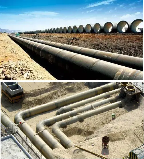
Underground or buried piping (or Pipeline) is all piping that runs below grade. In every process industry, there will be some lines (Sewer or drainage system, Sanitary, and Storm Water lines, Firewater or drinking water lines, etc), part of which normally runs underground. However the term buried piping or underground piping, in a true sense, appears for the pipeline industry as miles of long pipe run carrying fluids will be there.
Analysis of Underground Piping System
Analyzing an underground pipeline is quite different from analyzing plant piping. Special problems are involved because of the unique characteristics of a pipeline, code requirements, and techniques required in the analysis. Elements of analysis include pipe movements, anchorage force, soil friction, lateral soil force, and soil pipe interaction.
Fig. 0 Typical Buried Piping
Why Pipeline Stress Analysis is different from Piping Stress Analysis?
To appreciate pipe code requirements and visualize problems involved in pipeline stress analysis, it is necessary to first distinguish a pipeline from plant piping. Unique characteristics of a pipeline include:
High allowable stress of Pipeline
A pipeline has a rather simple shape. It is circular and very often runs several miles before making a turn. Therefore, the stresses calculated are all based on simple static equilibrium formulas which are very reliable. Since stresses produced are predictable, the allowable stress used is considerably higher than that used in plant piping.
High-yield strength pipe
To raise the allowable, the first obstacle is yield strength. Although a pipeline operating beyond yield strength may not create structural integrity problems, it may cause undesirable excessive deformation and the possibility of strain follow-up. Therefore, a high test line with a very high yield to the ultimate strength ratio is normally used in pipeline construction. The yield strength in some pipes can be as high as 80 percent of ultimate strength. All allowable stresses are based only on yield strength.
The movement of the pipeline is normally due to the expansion of a very long line at the low-temperature difference. Pressure elongation, negligible in the plant piping, contributes much of the total movement and must be included in the analysis.
Soil-pipe interaction
The main portion of a pipeline is buried underground. Any pipe movement has to overcome soil force, which can be divided into two categories: Friction force created from sliding and pressure force resulting from pushing. The major task of pipeline analysis is to investigate soil-pipe interaction which has never been a subject in plant piping analysis.
Low Design Temperature
Normally these lines do not have high design temperatures (of the order of 60 to 82 degrees centigrade) and only thermal stress checking is sufficient for the underground part. Common materials used for underground piping are Carbon Steel, Ductile iron, cast iron, Stainless Steel, and FRP/GRP.
In this article, I will try to explain the steps followed while analyzing such systems using Caesar II. However, this article does not cover the basic theory for analysis.
Inputs Required for U/G Pipe Stress Analysis
Before proceeding with the analysis of buried piping using Caesar II collect the following information from the related department
Isometric drawings or GA drawings of the pipeline from the Piping layout Department.
Line parameters (Temperature, Pressure, Material, Fluid Density, etc) from the Process Department.
Soil Properties from the Civil Department.
Caesar II for Underground Piping Analysis
The CAESAR II underground pipe modeler is designed to simplify user input of buried pipe data. To achieve this objective the “Modeler” performs the following functions for analysts:
Allows the direct input of soil properties. The “Modeler” contains the equations for buried pipe stiffnesses that are outlined later in this report. These equations are used to calculate first the stiffnesses on a per length of pipe basis, and then generate the restraints that simulate the discrete buried pipe restraint.
Breaks down straight and curved lengths of pipe to locate soil restraints. CAESAR II uses a zone concept to break down straight and curved sections. Where transverse bearing is a concern (near bends, tees, and entry/exit points), soil restraints are located in close proximity, and where axial load dominates, soil restraints are spaced far apart.
Allows the direct input of user-defined soil stiffnesses on a per-length-of-pipe basis. Input parameters include axial, transverse, upward, and downward stiffnesses, as well as ultimate loads. Users can specify user-defined stiffnesses separately, or in conjunction with CAESAR II’s automatically generated soil stiffnesses.
Modeling steps followed in Caesar II
The modeling of buried piping is very easy if you have all the data at your hand. The following steps are followed for modeling:
From the isometric model, the line is in the same way as you follow in the case of an above-ground pipe model i.e, enter line properties in Caesar Spreadsheet, enter lengths by breaking the line into several nodes, or select an existing job for converting it into an underground model.
The analyst can start the Buried Pipe Modeler by selecting an existing job and then choosing Input-Underground from the CAESAR II Main Menu. The Modeler is designed to read a standard CAESAR II input data file that describes the basic layout of the piping system as if it was not buried. From this basic input, CAESAR II creates a second input data file that contains the buried pipe model. This second input file typically contains a much larger number of elements and restraints than the first job. The first job that serves as the “pattern” is termed the original job. The second file that contains the element mesh refinement and the buried pipe restraints is termed the buried job. CAESAR II names the buried job by appending a “B” to the name of the original job.
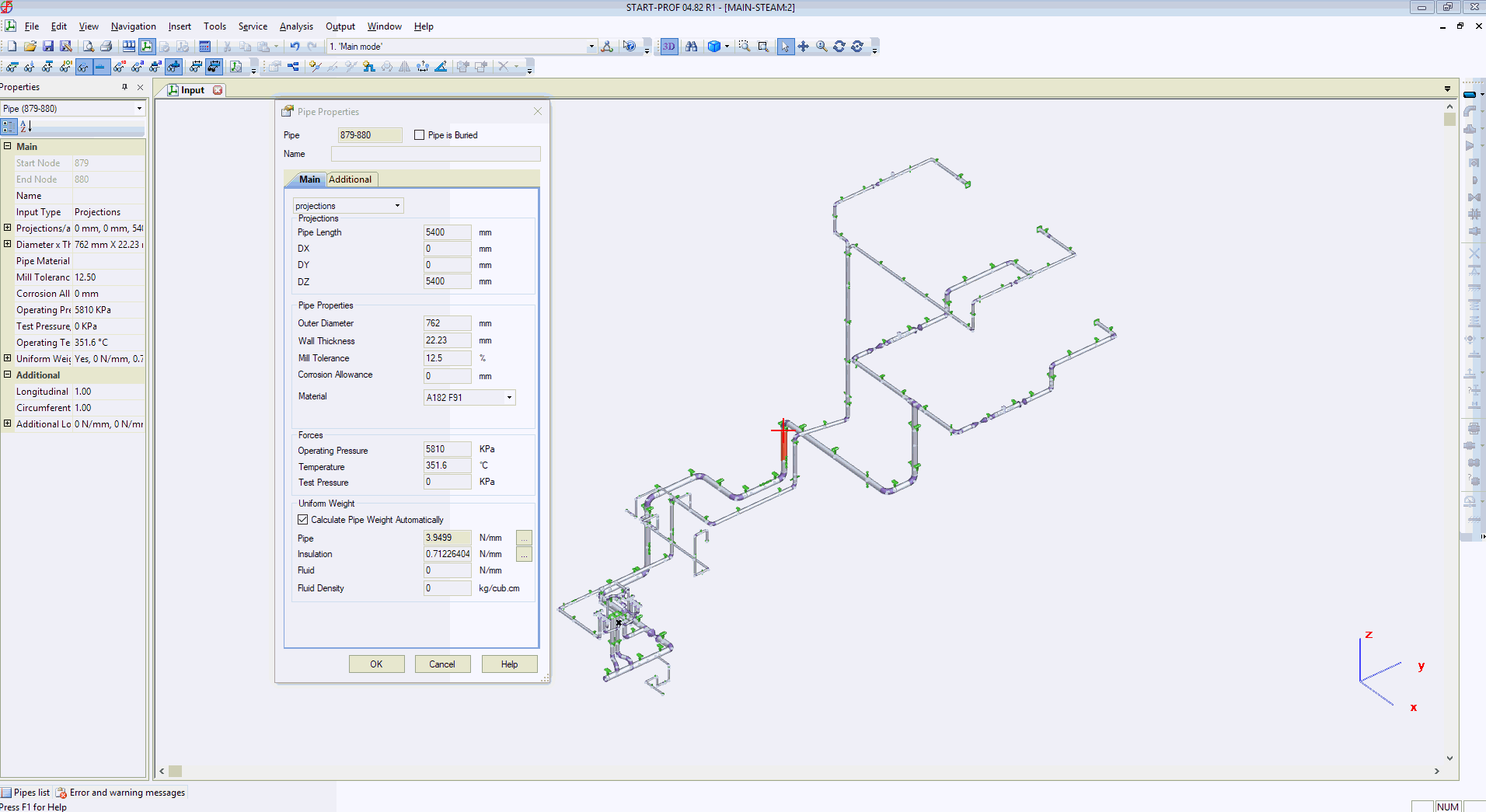
When the Buried Pipe Modeler is initially started up, the following screen appears:
Fig. 1: Sample Caesar II Spreadsheet for Buried Piping
This spreadsheet is used to enter the buried element descriptions for the job. The buried element description spreadsheet serves several functions:
It allows the analyst to define which part of the piping system is buried.
Allows the analyst to define mesh spacing at specific element ends.
Allows the input of user-defined soil stiffnesses.
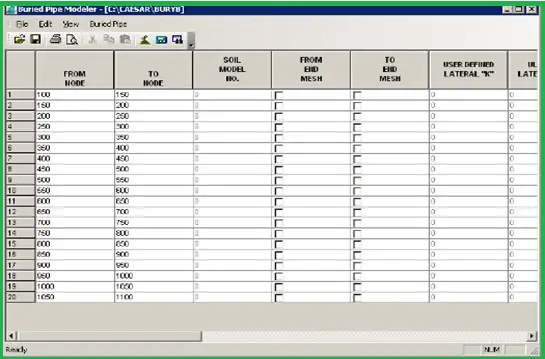
From/ To node
Any element of pipe in CAESAR II can be defined by two elements first is a start point and the second is an endpoint. In the buried pipe model, before conversion, the From/ To nodes remain the same as in the unburied model.
Soil model No
This column is used to define which of the elements in the model are buried. A nonzero entry in this column implies that the associated element is buried. A 1 in this column implies that the analyst wishes to enter user-defined stiffnesses, on a per-length-of-pipe basis, at this point in the model. These stiffnesses must follow in columns numbers 6 through 13. Any number greater than 1 in the soil model no. column points to a CAESAR II soil restraint model generated using the equations outlined later under Soil Models from analyst-entered soil data.
From/ To mesh type
A critical part of the modeling of an underground piping system is the proper definition of Zone 1 bearing regions. These regions primarily occur:
On either side of a change in direction
For all pipes framing into an intersection
At points where the pipe enters or leaves the soil
CAESAR II automatically puts a Zone 1 mesh gradient at each side of the pipe framing into an elbow. Note it is the analyst’s responsibility to tell CAESAR II where the other Zone 1 areas are located in the piping system.
User-defined stiffness & ultimate load
There are 13 columns in the spreadsheet. Columns 6 to 13 carry the user-defined soil stiffnesses and ultimate loads if the analyst defines soil model 1. The analyst has to enter lateral, axial, upward, and downward stiffnesses & loads.
Procedure
Select the original job and enter the buried pipe modeler. The original job must already exist and will serve as the basis for the new buried pipe model. The original model should only contain the basic geometry of the piping system to be buried. The modeler will remove any existing restraints (in the buried portion). Add any underground restraints to the buried model. Rename the buried job if the CAESAR II default name is not appropriate.
Enter the soil data using Soil Models.
Describe the sections of the piping system that are buried, and define any required fine mesh areas using the buried element data spreadsheet.
Convert the original model into the buried model by the activation of option Convert Input. This step produces a detailed description of the conversion.
Exit the Buried Pipe Modeler and return to the CAESAR II Main Menu. From here the analyst may perform the analysis of the buried pipe job.
Online Video Course on Buried/Underground Piping/Pipeline System Stress Analysis
If you need to join an online buried pipe stress analysis course using Caesar II to learn the above using a practical case study then click here to join the same.
Refineries and petrochemical plants obtain feedstocks and dispatch products in a number of ways. The most common methods are by pipeline, road, rail, and sea. A marine import/export facility is a very important item for a refinery or petrochemical plant. Under-design of the marine facilities can result in process plant throughput being constrained. Over-design can lead to a substantial increase in capital cost, which can have a significant effect on the overall economics of a Project.
Whereas the majority of process unit operations are continuous processes, marine loading/unloading is always a batch operation. It is therefore most important that all the requirements and activities associated with the start-up and shutdown of each type of loading/unloading operation are covered in the specification/design of marine facilities. This article will assist process engineers with the design of facilities for importing feedstocks and exporting products by sea. This document covers the key process design issues associated with the design/specification of marine systems, including jetties/berths, single-point moorings, and the associated loading systems.
Marine System design guidelines
The following guidelines can be followed during the design of a marine system
At an early stage of the design of a marine facility, an estimate of the throughput of each material to be handled and the capacities of tankers that will transport them must be agreed upon by all parties, as a starting point for the design work. This information is fundamental to the design.
Initial Estimate of Number of Berths Required- When throughput/tanker size data has been agreed upon, it is recommended that an initial estimate is made of the number of berths required.
Types of Berth
Berths can be divided into the following categories:
Single Point Mooring (SPM): Feedstocks/products are pumped via sub-sea pipeline(s) from/to a tanker that has moored up to a floating buoy, located off-shore.
Single Berth: One berth, either on a jetty or on the quayside, normally with multiple loading arms for one tanker to load/unload products/feedstocks
Multiple Berths, forming a harbor: A number of berths, normally on a jetty, enabling several tankers to load/unload products/feedstocks simultaneously
SPMs are favored when the maximum tanker size is such that dredging and/or a very long jetty structure would be required to provide sufficient draught i.e. when large tankers have to be accommodated. Single berths are seen most often in deep water locations and in river estuaries.
Location of Shipping Tanks / Pumps
In some cases, a Client may not have finalized the location of the product (or feedstock) tank farm before the design work starts. In such cases, it should be noted that pumping to/from tankers is generally at much higher flow rates than the rates at which feedstocks/products are consumed/produced by a process plant. Hence the pumps/pipelines etc. serving marine systems are generally much larger than the pumps/pipelines connecting process plants to storage tanks. For this reason, in cases where there is a significant distance between a process plant and the supporting marine facilities, it is more economic to locate the shipping tanks/pumps close to the marine facilities, rather than close to the process plant.
Segregation of Feedstocks / Products
It is important to ensure that marine loading facilities are designed to segregate products/feedstocks. Segregation is best achieved by designing dedicated marine facilities for each material. But this is often impractical or uneconomic. At a multiproduct berth, it is normal for loading arms to be used for several similar products. If economics dictate that pipelines must be multi-product (e.g. when the marine loading facility is a long way from the export tanks), flushing or pigging facilities (or a system to detect and slop the interface material) are required.
Types of Tankers/ Tanker Types in a Marine System
Broadly speaking tankers can be classified as either conventional, pressurized, refrigerated, or semi-refrigerated. For all tanker types, onshore pumps are used for loading, and onboard pumps are used for unloading. Key features of these types of tanker are as follows:
A conventional tanker carries fluids with true vapor pressures of less than one atmosphere minus a suitable safety margin. This margin tends to vary slightly between clients and carriers, but usually, the maximum vapor pressure is approximately 0.75 atm. The tanker comprises a number of compartments that can be filled or emptied independently. Most tankers also have slop tanks, separate from the product tanks. Tankers carrying highly flammable or oxidizable materials often have inerting facilities, by which exhaust gases from the tanker’s engines are passed into the vapor space in the tanks.
Pressurized liquid gas tankers usually have fewer storage compartments than conventional tankers. The smaller one might comprise a single-pressure container. It is usual for pressurized liquid gas tankers to use a vapor connection for the transfer of displaced vapor at both the import and export locations.
Refrigerated gas tankers are usually bigger than pressurized tankers. They generally have more compartments and can withstand little pressure. The refrigeration plant on board is usually designed to counter heat in leak only, hence only liquids that are fully cooled can be loaded.
Semi-refrigerated tankers are sometimes used, and these combine the attributes of both pressurized and refrigerated tankers.
It should be noted that the maximum operating pressure of pressurized and semi-refrigerated tankers varies from vessel to vessel. The metallurgy of refrigerated and semi-refrigerated tankers governs the minimum temperature allowed and hence the products that can be handled.
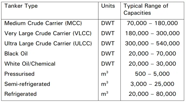
Marine System Tanker Capacities/ Capacities of tankers
It should be noted that when designing a terminal, the number and volume of feed/product tanks are required to depend to a great extent on the range of tanker capacities that have to be accommodated. The capacity of a tanker that carries material at ambient conditions is generally given in Dead Weight Tonnes (DWT). The capacity of a tanker that carries refrigerated or pressurized material is generally given as a volume. Typical ranges of tanker capacities are as follows:
Fig. 1: Tanker Types vs Capacities
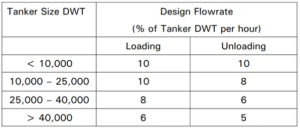
Tanker Loading and Unloading Rates:
Typical loading/unloading rates for tankers are as follows:
Fig. 2: Tanker Size vs Design flowrate
Even if the
design loading/unloading rates for the specified tankers are appreciably less
than the figures given above, it is recommended that these design
loading/unloading rates are used (for the purposes of hydraulic design, but not
for the purposes of calculating the berth occupancy) to give the marine
terminal flexibility and provide a robust design.
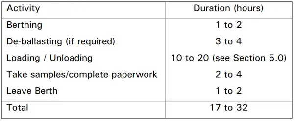
Berth Turnaround Time for Marine System design
The Berth Turnaround Time is a term often used to describe the total elapsed time from the moment a tanker starts its approach to a berth, to the moment that the tanker is clear of the port area, thereby allowing another tanker to begin its approach. Realistic time intervals for a tanker using a berth or jetty are as follows:
Fig. 3: Berth Turnaround Time
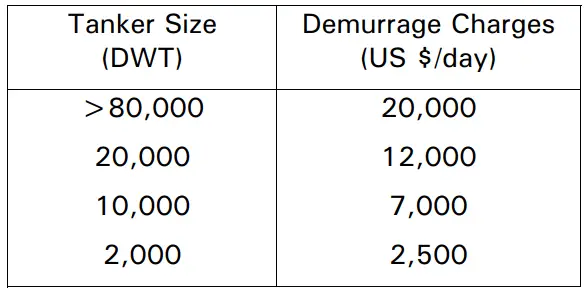
Demurrage/ Berth Occupancy
Demurrage is a
charge paid by the Refinery/Petrochemical plant operator to the ship
operator/owner in the event of a tanker being delayed. Examples of circumstances in which demurrage
fees are payable include:
A tanker arrives at a marine
facility on schedule, but there is no berth available for the tanker.
A tanker starts loading as
scheduled, but for reasons outside the tanker captain’s control, the loading
operation takes longer than the pre-agreed maximum time.
Demurrage fees are charged on a daily basis and can become a very significant operating cost. During the design of a marine facility, berth occupancies should be calculated for various scenarios, in order to reduce/minimize demurrage charges. In practice, it is not possible to avoid incurring some demurrage charges, without over-designing the marine facility. As a very rough guide, the following demurrage costs can be used, but the actual costs should be provided by the Client or a marine consultant.
Fig. 4: Tanker Size vs Demurrage Charges
Single Point Mooring (SPM) Systems
SPMs provide a useful method of loading/unloading tankers from/to onshore facilities when it is not practicable to build a jetty. Jetties tend to be impracticable in shallow water (e.g. in estuaries or on continental shelves) when loading/unloading deep-drafted vessels. SPMs are also appropriate in deepwater locations.
The concept of the SPM is simple. The tanker approaches the mooring from the down current. The bow is made fast to the buoy. With the main engines stopped, the tanker now hangs from the buoy with the bow into the current as required. If there is a change of current (or wind) direction, the tanker swings freely around the buoy (known as weather vaning).
Floating hoses from the buoy are hoisted to the tanker’s manifolds and connected, thus permitting loading/unloading. The buoy is connected by the subsea pipeline to the storage facilities. The hoses have to be connected to the pipeline by a swivel so full 360º movement of the tanker can be accommodated without interfering with hose operation.
Jetty Topside Facilities
Jetty topside
facilities generally include some/all of the following equipment items/systems:
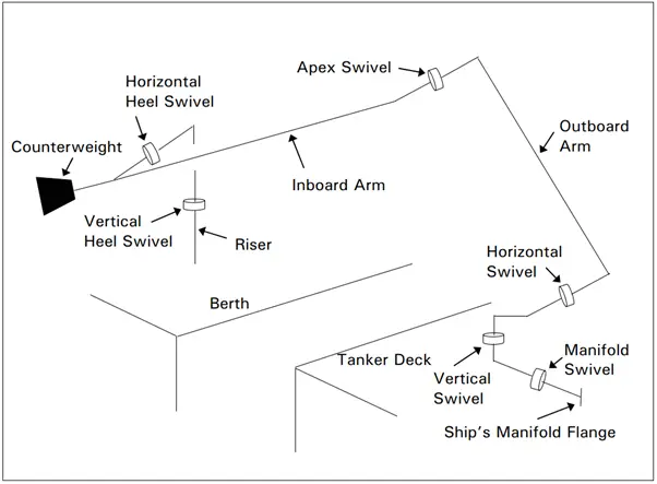
Loading arms are made up of several sections of pipe, connected by swivel joints. The section on the shore side of the ‘apex’ of the loading arm is known as the inboard arm and the section on the tanker side of the ‘apex’ is known as the outboard section. See the following Figure for a diagram of a loading arm.
When loading/unloading tankers, accurate metering is normally a requirement, for both custodial and regulatory reasons. Metering with sufficient accuracy can be achieved using either tank gauging or certain types of flowmeter.
Deballasting Facilities
Most tankers have to be partially filled with ballast water when they are not carrying cargo, in order to make the tankers seaworthy i.e. stable in rough weather. Seawater is generally used as ballast water.
Surge
Marine loading/unloading systems are often designed to pump at high flow rates over large distances. Hence surge pressures (eg due to the closure of a MOV or a pump trip) can be large. It is most important that during detailed design, a surge analysis is carried out on each marine loading pipeline. Peak surge pressures should be calculated for all likely scenarios, to check that the design pressure of pipework/equipment (plus an allowance for short-term over-pressure) is not exceeded, even in the worst case.
VOC Recovery/Disposal
When loading products that are stored at ambient conditions, it is common for the displaced vapor to be simply vented into the atmosphere, thereby emitting volatile organic compounds (VOCs) into the environment. For very low vapor pressure products, the number of VOCs emitted by a tanker when loading is small if not negligible. But for a high vapor pressure product, such as motor gasoline and naphtha, a significant amount of product can be lost to the atmosphere, such as VOCs.
Drainage at Births
It is common to have a curbed area at each berth, in order to catch any material which may leak from, for example, the couplings on loading arms. The curbed area drains into a sump tank located below the berth on the jetty structure. The sump tank includes pumps that return the drainings to a slop oil tank or a ballast water tank or alternative disposal onshore.
Fire Detection and Protection
Remote-controlled monitors and hydrants are commonly provided at each berth, to fight a fire and to protect equipment from the effects of the fire. The fire may be at the berth/on the jetty or on the tanker at the berth. It is normal practice for a jetty/berth to have water sprays/water curtains to protect the structure/equipment and to provide means of escape for personnel in case of fire. It is common to provide valved connections on a fire main in the vicinity of a jetty, to enable a fire tug to connect up and pump water into the system, as a standby.
Valve selection is the process of choosing the appropriate valve for a specific application based on various factors such as the type of fluid or gas being handled, the operating conditions, and the required performance characteristics.
Valves are mechanical devices used to regulate the flow of fluids or gases in a piping system, and proper valve selection is crucial to ensure the safe and efficient operation of the system. The selection of a valve should take into consideration several factors, including the flow rate, pressure, temperature, and chemical compatibility of the fluid or gas being handled, as well as the required level of control or regulation.
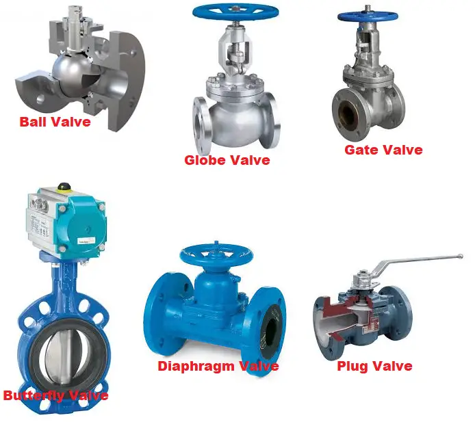
The type of valve selected can also affect the performance of the system, as different valves have different characteristics, such as flow capacity, pressure drop, and shut-off capability. Common valve types include ball valves, globe valves, gate valves, butterfly valves, and check valves, each with its unique features and benefits.
In addition to considering the fluid or gas properties and operating conditions, valve selection may also involve evaluating factors such as cost, reliability, ease of maintenance, and compatibility with other system components. Working with a qualified valve supplier or engineer can help ensure that the appropriate valve is selected for the specific application and that it meets all necessary safety and performance standards.
Valves are important mechanical (sometimes electro-mechanical) devices that help in controlling the fluid flow through pipes or tubes. Selecting the right kind of economic valve for a specified fluid service requires many considerations. This article provides guidelines for the selection of normal-type valves. (Special-type valves are not covered in this article).
It should be recognized that Valve Selection is a very extensive and complex subject and it is not possible to select only one type based on this article. The valve selected to work under the same conditions will differ from one client to another. It is necessary to compare the cost and come to an agreement with the client.
Fig. 1: Valves in Operating Plants
Criteria for Valve Selection
The selection of valve type requires an understanding of the following.
Valve Function
Service Characteristics
Cost of Valve
Valve Selection Based on Valve Function
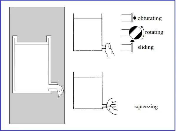
There are two basic principles by which valves are constructed.
(1) The first principle is developed in three ways:
Moving the stopper by direct thrust onto the orifice seating. This obturating movement is the basis of globe valves.
Sliding the stopper across the face of the orifice seating. This is the basis of gate valves.
(2) The second principle, squeezing action, is the basis of all diaphragm valves.
These are shown in the following Figure (Fig. 2)
Fig. 2: Squeezing Action for Diaphragm Type Valves
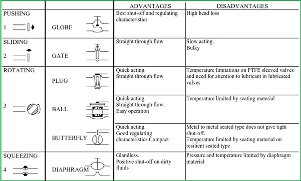
(3) Each of the four-valve motivations has its own advantages and disadvantages, as listed in the following table (Fig. 3).
Fig. 3: Table comparing the valve features
To summarize, there are four basic valve types, each type having its own individual characteristics and offering its own particular advantages or disadvantages.
For this reason, many modifications and variations of the basic type are made by valve manufacturers. An appraisal of the chief characteristics of the above four basic valve types is given in the following paragraphs
Globe Valve Selection Criteria
The globe valve is used for flow regulation or as a block valve where resistance to flow is not critical and positive closing action is required. They have a tortuous configuration which is typical of the closing method and results in higher resistance to flow compared with other valves.
Gate Valve Selection
Gate valves are used for on/off operation on hydrocarbon, general process, and utility services for all temperature ranges.
They have straight-through configurations which are typical of the sliding method, therefore, minimum resistance to flow.
The disadvantages are that they have the slowest action of all valves because the gate has to be moved a distance greater than the bore of the valve, which also means that the valve is of necessity bulky in height.
Selection of Plug valve
Plug valves have a quarter-turn operation, plugs are tapered or parallel plugs, and are suitable for most on-off clean processes and utility services, including non-abrasive slurries.
They have straight-through configurations typical of the sliding method.
The disadvantages of the basic plug cock are two-fold.
Firstly, its quick action can lead to a water hammer on hydraulic installation when it is closed too rapidly, and secondly, it is difficult to combine tight shut-off with ease of operation.
A low torque, quarter-turn, rotary action valve with a straight-through flow configuration in which the disc is turned through 90 degrees, close to open position, in axial turning bearings and is used as a control or block valve. It is of compact design and may be obtained with or without flanges and linings. The seating arrangement may be soft (use of body lining, trapped ‘O’ ring, etc.) or metal to metal.
When to Select the Diaphragm Valve
Diaphragm valves have straight-through flow or weir configurations employing the flexing method and may be used for low-pressure chemical plant processes on-off or regulating the operation of most gases and liquids, e.g. slurries, viscous fluids, and fluids that are chemically aggressive.
The inherent disadvantage is that the diaphragm has to be made from an elastomeric material, usually either a natural or synthetic rubber, and this limits the application of the valve with respect to both temperature and pressure. Also, because of the stresses induced in the diaphragm, the valve has a shorter working life than other valve types.
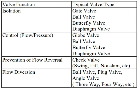
Typical Valve Types
Typical valve types for various operating functions are given in the following table.
Fig. 5: Valve Selection Based on Function
Valve Selection based on Service Characteristics
Valve selection is dependent on the characteristics of the services as follows.
Fluid type
Fluid characteristics
Pressure and temperature limitations
Operation and maintenance requirements
1. Fluid Type:
The fluid being handled should be classified as follows,
Liquid (including Two-Phase)
Gas
Steam
Slurry
Solids
2. Fluid Characteristics:
The characteristics and condition of fluids and slurries require careful identification since these are often the most significant factors in selecting the correct type of valve.
Clean fluids generally permit a wide choice of valve types, for dirty fluids the choice is often restricted and may require a specific type of valve.
The fluid is divided into the following characteristics.
(1) Clean Service
(2) Dirty Service
Dirty service involves fluids with suspended solids that may seriously impair the performance of the valve unless the correct type of design is selected. This type of service is often of major significance since many valves are very sensitive to the presence of solids. Dirty service is further classified as abrasive or sandy.
Abrasive Service is a term used to identify the presence of abrasive particulate found in piping systems and includes the presence of pipe rust, scale, welding slag, sand and grit which are damaging to many valves. These materials can damage seating surfaces and clog working clearances in valves often resulting in excessive force required to operate valves, sticking, jamming, and leakage through the valves.
Sandy service is a term identifying severe abrasive and erosive conditions and is used in oilfield production to identify the production of formation sand with reservoir crude oil or gas.
(3) Slurry Service
Slurry service involves liquids with substantial solids in suspension.
Slurries vary widely in nature and concentration of solids, and hard abrasive solids of high concentration can cause severe abrasion, erosion, and clogging of components.
Soft, non-abrasive solids can cause clogging of components.
In certain chemical processes, polymerization may block the cavities, preventing valve operation.
(4) Solids
There are many other conditions where solids may be present in the form of hard granules, crystals, soft fibers, or powders.
The transporting media may be liquid or gas. Air or fluidized bed systems may be used for some particulate. Specialized valves are available for many of these services but development work may sometimes be necessary.
(5) Hazardous & Flammable Service
Hazardous and flammable material is normally specified in Fire Service Law and/or the Client’s specifications.
Toxic substances such as chlorine, hydrofluoric acid, hydrogen sulfide, CO, phenol, etc.
Highly corrosive fluids such as acids and caustic alkalis.
(6) Corrosive Service
Corrosive service is a term generally used to identify clean or dirty fluids containing corrosive constituents that, depending on concentration, pressure, and temperature, may cause corrosion of metallic components. Corrosive fluids include sulfuric acid, acetic acid, hydrofluoric acid (HFA), wet acid gas (wet CO2), sour gas (wet H2S), and chlorides. Many chemicals are highly corrosive.
The choice of suitable corrosion-resistant materials for valve pressure retaining components (boy bonnet) and trim is necessary to avoid corrosion that can impair the integrity or performance of the valve.
(7) Viscous Service
Viscous service is a term that generally identifies a wide range of dirty or clean fluids with pronounced thickness and adhesive properties that, for the range of operating conditions(pressure, temperature, and flow) may require high operating torques and cause a sluggish response affecting seating. Fluids include high-viscosity oils (lube and heavy fuel oil) and non-newtonian fluids e.g. wax crude, gels, and pastes.
The choice of valves for viscous service can vary depending on fluid properties. Special attention should be given to the check valves where a sluggish response may cause operating difficulties and even hazardous conditions.
(8) Fouling Service
Fouling or scaling service involve liquids that form a deposit on surfaces. Such deposits may vary widely in nature, with varying hardness, the strength of adhesion, and rates of build-up. Valves for these services require careful selection, particularly where thick, hard, strongly adhesive coatings occur. The temperature of the fluid may be a vital factor and in some cases, valves may need tracing or be steam jacketed or of purged design.
(9) Solidifying Service
Solidifying service is a general term used to identify fluids that will change from liquid to solid unless maintained at the correct conditions of temperature, pressure, and flow. It is a term generally associated with fluids such as liquid sulfur and phthalic anhydride where valves of steam-jacketed design may be required or heavy fuel oil where valves often require tracing to maintain temperature and operability.
3. Pressure and Temperature Limitation:
Valves are normally allocated a rating according to the maximum operating pressure and temperature or the ratings of the piping system and flanges.
The temperature also limits the materials used in the valve construction, particularly the internals, trims, seals, rings, or lubricants.
These are normally defined in the “Piping Material Specification”.
4. Operation and Maintenance Requirements:
Operation and maintenance requirements can influence selection and design. Consideration should be given to:
Fire Resistance: There may be a requirement for valves having non-metallic (soft) seating to include ‘fire-safe’ features so that in the event of the soft seat and/or seals being damaged or destroyed by fire the valve will still be operational and any leakage will be within the acceptable limits laid down by a particular standard or specification.
Operability
Leak tightness (internal and external)
Maintainability
Storage and commissioning
Pipeline requirements (e.g. ability to pass cleaning pigs)
Valve Selection Considering the Cost of Valves
The costs of valve types cannot be simply compared because they vary depending on the countries where they are produced, vendors, and the balance of demand and supply.
In most cases, clients call for stress relieving, annealing, radiographic inspection, etc. of the valves, which affects the cost of the valves. Therefore, it is necessary to ask the Procurement Division to inquire about suitable vendors regarding these valves, based on the service conditions and the client’s requirements, after they are defined.
After a draft of the P&ID is issued, the personnel in charge of the preparation of the P&ID should cooperate closely with the piping design engineers in charge, during the in-house review period of the P&ID, and should determine the valve types and prepare piping material specifications in parallel.
Generally, gate valves are less expensive than globe valves of the same specification. However, the cost of 1-1/2″ or smaller-dia. malleable gate valves are higher than that globe valves.
Class 150 Gr.304SS TFE-seat 4” or smaller-dia. ball valves are less expensive than gate and globe valves.
Class 150 cast iron/malleable iron TFE-seat 2″-4″ ball valves are less expensive than gate and globe valves whose rating and material are the same.
In recent years, domestic vendors have developed and distributed light and inexpensive 2″ or smaller wafer-type ball valves, which should be positively adopted in chemical plants.
The cost of soft-seat butterfly valves, applied in the range of approximately 10 kg/cm and 80°C or lower, is the lowest compared with other types of valves.
Metal-seat butterfly valves could be used in the same applicable range as general gate valves if the same material is used for the metal seat. Also, as Class 600 and 900 butterfly valves have been developed and distributed, they should be positively applied to process lines. If the butterfly valves are throttled in use, care should be taken to avoid cavitation.
Valves are one of the important mechanical (sometimes electro-mechanical) device that helps in controlling the fluid flow through pipes or tubes. Selecting the right kind of economic valve for a specified fluid service requires many considerations. This article provides guidelines for the selection of normal type valves.
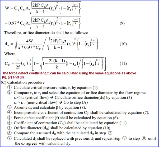
Guidelines for Sizing of Restriction Orifice for Single-phase Fluids
Of many kinds of flow restriction devices, restriction orifices (RO) are frequently used, because they are simple and economical devices. RO is applied to regulate the flow rate or pressure. This article will provide the guidelines for the sizing of the Restriction Orifice. It should be noted that this standard practice is applicable to single-phase fluids only.
Inputs Required for Restriction Orifice Sizing
The following is a summary of input data to be prepared for the design of RO:
For vapor service: molecular weight, Cp/Cv, Z-factor, viscosity
(3) Minimum allowable value of cavitation index for liquid service
Output from the Restriction Orifice Design
(1) Single orifice
Orifice diameter
The pressure at vena-contracta
Velocity at orifice
Calculated cavitation index (for liquid)
Critical or non-critical (for vapor)
(2) Multi-stage orifice
Required stage number
Orifice diameter of each orifice
Distance between adjacent orifice plates
Inlet and outlet pressures of each orifice
The pressure at vena-contracta of each orifice
Velocity at each orifice
Calculated cavitation index of each orifice
Principles of RO Sizing Calculation
Flow restriction orifice calculation for Gas Service
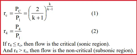
Critical Pressure Ratio:
The critical pressure ratio, rc can be obtained from the following equation.
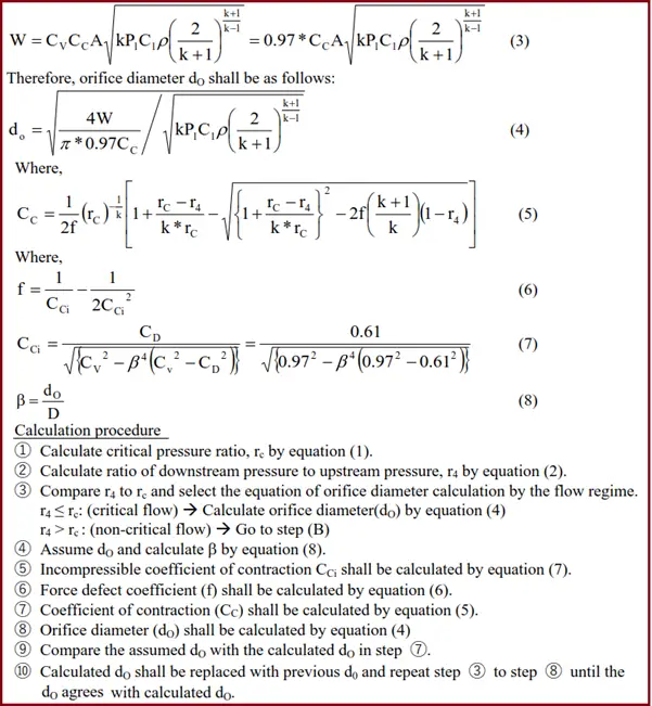
Orifice Diameter:
The equation for orifice diameter should be selected using equation (2), depending on whether the flow is critical or non-critical.
(A) Critical flow (sonic region)- When the ratio of downstream pressure to upstream pressure, r4, is smaller than or equal to the critical pressure ratio, rc, the following equation of orifice diameter for a critical flow should be used.
(B) Non-critical flow (subsonic region)- The following equation of orifice diameter can be used for the non-critical flow region.
Restriction orifice calculation for Liquid Service:
Orifice Diameter:
Cavitation Index
In order to avoid the cavitation problem, the minimum allowable value of the cavitation index, Kd, should be selected based on the following:
(1) Cavitation index Kd=0.37 shall be used for the usual case. At this critical cavitation condition, the noise is steady but still light. No erosion will occur. (Once the orifice chokes and supercavitation occurs, no damage by erosion will exist near the orifice. This is because the damage is caused by the collapse of the cavities and the collapse occurs far downstream during supercavitation)
(2) On some occasions such as in the following cases, use Kd=0.93 as an incipient cavitation condition in order to avoid severe economical risk.
Material is high grade such as stainless steel or higher and pipe size is larger than 12”.
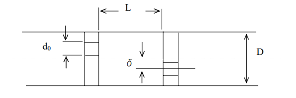
Interval of Orifices
In the case of the multi-stage restriction orifice, the minimum distance, as shown below, should be provided between orifices, to avoid a reduction in RO performance.
For concentric orifice: L ≥ 5.4*D*(1-β)
For eccentric orifice: L ≥ D
Deflection Ratio of Eccentric Orifice
The deflection ratio of the eccentric orifice “e” is 0.75.
e = 2δ /(D − d0 ) = 0.75 (14)
Where,
δ: Pipe center to orifice center length (m)
d0: Orifice hole diameter (m)
D: Pipe inside diameter (m)
Image showing Deflection Ratio for Eccentric Orifice
① Decide the minimum allowable value of the cavitation index to meet a given situation.
Kd = 0.37: for the usual case
Kd = 0.93: for the conservative case
② Assume dO and calculate β by equation (8).
③ Incompressible coefficient of contraction CCi shall be calculated by equation (7).
④ Orifice diameter (dO) shall be calculated by equation (13).
⑤ Compare the assumed d0 with the calculated dO in step ④.
⑥ Calculated dO shall be replaced with the previous dO and repeat step ② to step ⑤ until the dO agrees with the calculated dO.
Calculate the cavitation index, Kd by equation (15), and compare it with the minimum allowable value.
If the cavitation index ≥ 0.37 (or 0.93), then the orifice diameter is acceptable.
If the cavitation index < 0.37 (or 0.93), then a single orifice is unable to accommodate the required pressure drop. In that case, a multi-stage orifice system should be applied.
B. Multistage Restriction Orifice Calculation
① Decide the minimum allowable value of the cavitation index to meet a given situation.
Kd = 0.37: for the usual case
Kd = 0.93: for the conservative case
First stage orifice: located at the outlet
② Assume upstream pressure of the first stage orifice.
③ Assume dO and calculate β by equation (8) for the first stage orifice.
④ Incompressible coefficient of contraction CCi shall be calculated by equation (7).
⑤ Orifice diameter (dO) shall be calculated by equation (13) using assumed upstream pressure.
⑥ Compare the assumed d0 with the calculated dO in step ⑤.
⑦ Calculated dO shall be replaced with the previous dO and repeat step ③ to step ⑥ until the dO agrees with the calculated dO.
⑧ Calculate cavitation index, Kd, using Equation (15), and compare with minimum allowable value.
If the cavitation index > 0.37 (or 0.93), increase the upstream pressure and repeat the steps from ③ to ⑧.
If the cavitation index < 0.37 (or 0.93), decrease the upstream pressure and repeat the steps from ③ to ⑧.
If the cavitation index equals or slightly bigger than 0.37 (or 0.93), the design of the first stage RO is completed and go to step ⑨.
n-th stage orifice
⑨ Set the upstream pressure of (n-1)-th stage orifice for the downstream pressure of the n-th stage orifice.
⑩ Assume the upstream pressure of the n-th stage orifice.
⑪ Repeat the steps from ③ to ⑧, until the cavitation index is equivalent to the minimum allowable value.
Special Consideration of RO Design:
(1) The minimum hole diameter of RO-
To prevent the plugging problem with RO caused by debris, the hole diameter should be greater than the following values:
For the clean liquid service: 2mm
For the clean Gas service: 1mm
When a diameter smaller than the above values is required, the strainer or filter to remove debris should be provided upstream of RO.
(2) The necessity of minimum straight run length-
Basically, the objective of RO is rough control of the flow rate and should not be used for strict control of the flow rate. Therefore, it should not be necessary to take a straight run of piping both upstream and downstream of RO to keep performance. However, for erosional services such as slurry or flush services, countermeasures for erosion shall be considered.
(3) The calculated hole diameter of RO should be rounded to the conservative size for easy manufacturing.
Restriction Orifice Sizing Spreadsheet
A restriction orifice sizing spreadsheet is an electronic tool or software program that helps in calculating the size of a restriction orifice based on various parameters such as flow rate, fluid properties, pressure drop, and pipe dimensions. Often they may come in the form of restriction orifice calculation excel.
Restriction orifices are used in piping systems to control the flow rate of a fluid, and their proper sizing is crucial for the system’s safe and efficient operation. A restriction orifice sizing spreadsheet typically uses industry-standard equations and formulas to calculate the required orifice diameter and other necessary parameters.
The input parameters required for the calculation typically include fluid density, viscosity, pressure, temperature, pipe diameter, and the desired pressure drop across the restriction orifice. The spreadsheet then calculates the required orifice diameter and other related parameters such as Reynolds number, velocity, and flow rate.
The use of a restriction orifice sizing spreadsheet can simplify the orifice sizing process and reduce errors associated with manual calculations. However, it is essential to use reliable and accurate spreadsheet templates or software programs and to validate the results obtained from the spreadsheet against industry standards and guidelines.