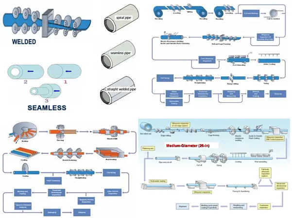
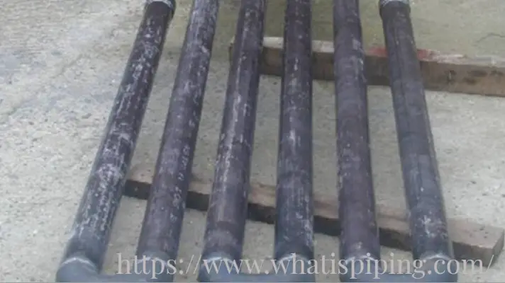
Seamless pipe is made from a round steel billet (solid cylindrical hunk of steel that is cast from raw steel). This billet is then heated, stretched out, and pushed or pulled over a form. It is then pierced through the center with a die and mandrel which increases the inside diameter and reduces the outside diameter. Even though seamless pipes are manufactured in a variety of sizes, with an increase in pipe diameter the production cost increases. The name seamless comes from its absence of a seam. Seamless pipes are widely used in process piping, power piping, shipbuilding, pressure vessel, construction, and chemical industries.
What is a Welded Pipe?
Welded pipe is made by cold forming flat strips, sheets, or plates into a round or circular shape by a roller or plate bending machine. The pipe is then welded with or without filler material using a high-energy source. Welded pipes can be produced in large sizes without any size restriction. Welded pipes are normally used for the transportation of water, oil, or gases in large quantities.
Fig. 1: Welded vs Seamless Pipe manufacturing
Seamless vs Welded Pipe
From the above paragraphs, it is obvious that seamless and welded pipes differ in their manufacturing process. The other differences are listed in the below-attached table.
Sr. No
Parameter
Seamless Pipe
Welded Pipe
1
Strength
Seamless pipes are able to withstand more pressure and load as there is no weak seam.
Due to welding, welded pipes are believed to withstand 20% less pressure and load as compared to seamless pipes.
2
Length
Seamless pipes are relatively shorter in length due to manufacturing difficulties.
Welded pipes can be manufactured in long continuous lengths.
3
Size
Seamless pipes are usually manufactured for a nominal size of 24 inches or less.
There is no such size restriction on welded pipe production.
4
Corrosion Resistance
Sealless pipes are less prone to corrosion means more corrosion-resistant.
The weld areas of the welded pipes are more prone to corrosion attacks, which means less corrosion resistance.
5
Surface Quality
The surface quality of seamless pipes is rough due to the extrusion process
Welded pipes have a smooth high-quality surface as compared to seamless pipes.
6
Economy
Costlier
More economic
7
Production Process
The production process of seamless pipe is quite complex with a long procurement lead time
The welded pipe production process is comparatively simpler with a short procurement lead time.
8
Tests
Seamless pipes do not require testing for weld integrity.
Welded pipes must be tested before use.
9
Application
Seamless pipes are widely suitable for high pressure, temperature, and corrosive environment
Welded pipes are normally used for less corrosive and low-pressure environments.
10
Availability
Less availability, limited material types, longer delivery time.
Readily available for various different materials; shorter delivery time.
11
Wall Thickness
Seamless pipes have inconsistent wall thickness across the length, thicker so heavier
Wall thickness for welded pipes is more consistent than seamless ones, thinner
12
Ovality
Seamless pipes provide better ovality, roundness
Welded pipes provide poor ovality and roundness as compared to their seamless counterpart.
13
Internal surface check
Checking not possible
The internal surface for welded pipes can be checked before manufacturing
Table explaining differences between Seamless and Welded Pipes
Pipe Selection, Welded or Seamless?
Even though improved manufacturing methods of recent times can produce welded pipes comparable to seamless pipes, still seamless pipes are preferred in a maximum of cases. However, for large-size piping applications, (> 24-inch NPS) welded pipes are mostly preferred due to less cost. Along with cost, various other parameters like diameter-to-thickness ratio, availability, corrosion resistance, etc. are considered for pipe selection.
Pump affinity laws or Pump Laws are used during hydraulic design to calculate the volume, capacity, head, or power consumption of the centrifugal pumps with changing speeds or wheel diameters. These laws are very important in pump design as they express the relationship between the variables that decide the pump performance.
The Pump affinity laws are basically a set of formulas that predict the impact of Change in Pump impeller Diameter and its Rotational Speed on the Pump Head (h), Pump Flow (Q), and Power Demand of the Pump (P). The affinity laws are applied both to centrifugal and axial flows. These laws can also be applied to fans and hydraulic turbines.
Uses of Pump Affinity Laws
Pump Affinity laws are widely used to predict the pump performance at a different speed or with different impeller diameters provided the pump performance curve at a certain speed or impeller diameter is known.
Using the series of ratios that pump affinity laws establish, a pump engineer can predict the performance of the pump subject to changing pump conditions. So, Pump affinity laws are a great tool to help pump engineers.
You can refer to our video article on the same subject by clicking here. To get an update regarding more similar videos please click here and subscribe to our channel.
Types of pump affinity law?
As mentioned above these laws study the impact of impeller diameter & rotational speed of the pump. Hence the affinity laws are framed
Once keeping the diameter constant (D=Constant) and
Once keeping the rotational speed constant (N=Constant).
So based on these conditions below mentioned are the cases and relations on flow, head & power consumption of the pump.
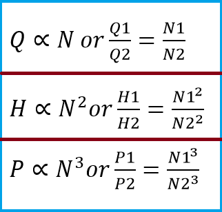
Pump Affinity law keeping the impeller diameter Constant
As per the first set of pump affinity laws for a given pump with a fixed impeller diameter:
The flow of the pump is directly proportional to the change in the speed of the pump. This means there will be the same amount of change in the flow of the pump as the rotational speed of the pump changes.
The Head of the pump is proportional to the square of speed. This means a change in pump rotational speed will lead to a change in the square root of the pump head.
Power is proportional to the cube of the speed. This means that when the rotational speed of the pump is increased the power consumption of the pump will be increased by 8 times.
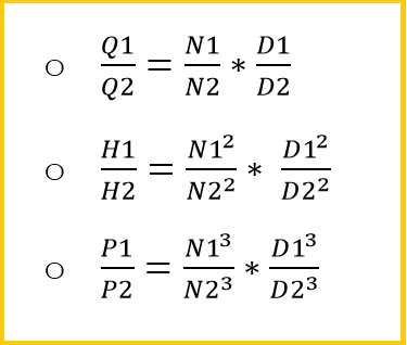
The above points can be presented mathematically as given below
Fig. 1: Affinity Laws with constant impeller diameter
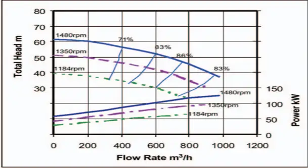
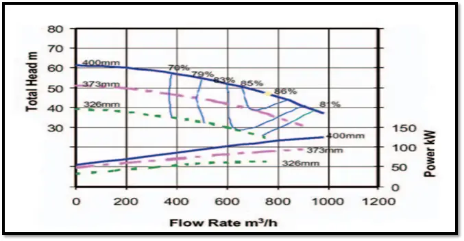
Fig. 2: Graphical representation of Pump Head vs Flow Rate
Normally, within the range of normal pump operational speeds, there is no appreciable change in efficiency. Because of this, the first Set of Pump Affinity Laws is reasonably accurate and reliable.
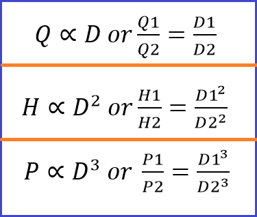
Pump Affinity laws keeping the pump speed constant
As per the second set of pump affinity laws for a given pump with a constant speed:
The flow of the pump (Pump Capacity) is directly proportional to the change in the impeller diameter of the pump. This means there will be the same amount of change in the flow of the pump as the impeller diameter of the pump is changed.
The Head of the pump is proportional to the square of the impeller diameter. This means a change in the pump impeller diameter will lead to a change in the square root of the pump head
Power is proportional to the cube of the impeller diameter. So, when the diameter of the pump is increased the power consumption of the pump will be increased by 8 times.
Mathematically the aforementioned points can be represented as given in Fig. 3.
Fig. 3: Affinity Laws with constant pump speed
Fig. 4: A typical pump performance curve
Note that, inaccuracies can be introduced into the predictions of the second set of pump affinity laws as efficiency changes with changes in impeller diameter.
Combined Pump Affinity Law
The flow, head, and power consumption of a pump change can be combined as shown in Fig. 5 when both rotational speed & impeller diameter change.
Fig. 5: Combined Pump Affinity Law
Example Calculation Explaining Pump Affinity Law
Consider a pump of flow 1000 m3/hr is designed for 1500 rpm. The same pump is required to be operated at 3000 rpm. Find the changed flow of the pump. Assume the diameter of the pump is kept constant.
Solution:
As per the pump affinity law when the impeller diameter is kept constant:
Q∝N or Q1/Q2=N1/N2; So, Q1 = 1000m^3/hr, N1 = 1500rpm, Q2 =? , N2 = 3000 rpm.
Hence, 1000/Q2=1500/3000; Q2=2000 m^3/hr
Hence for the same pumps if the RPM of the pump is doubled flow will also get doubled.
In the same example let’s take Power consumption = 100Kw, so find P2 at the changed RPM. P∝N^3 or P1/P2=(N1^3)/(N2^3 ) So, 100/P2=(1500^3)/(2000^3 ) Or P2 = 800 kW.
Hence a change in rpm will increase the power consumption of the pump 8 times.
Want to learn more. Here are a few Handpicked articles to add value to your learning process.
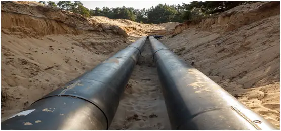
The piping that is in contact with soil or runs below grade level is called buried or underground piping. In the oil and gas industry, we find frequent use of buried piping mainly for cross-country pipelines where security and safety justify the pipelines to be underground. Here security means the difficulty of sabotage and intentional damage to an underground pipeline. Safety means the safety of the environment and the surrounding population centers due to accidental damage to the underground pipeline.
The firefighting system network piping mostly runs below ground with certain sections above-ground. Above-ground pipelines are also intermittently buried in roads and railway crossings. Other major applications include Cooling water lines inside process plants, Oily Water Sewer lines, Contaminated Rain Water Sewer from the process catchment area, Sanitary systems, Equipment drainage to slop tank, Closed Blow-Down system, Storm Water, Liquid Effluent to the Effluent Treatment Plant, etc.
However, note that Piping should not be buried or installed underground if it can be reasonably avoided.
A basic understanding of the concepts of buried piping installation along with routine process design calculations related to piping such as pressure drop, velocity and erosion/corrosion limits for various pipe metallurgies are always advantageous for engineers. This article will provide some important guidance on buried or underground pipe installation.
Underground Piping in Process Piping
In the process piping industry, underground piping falls into one of the following two categories:
Process lines &
Drain lines (Closed Process drains and Open Gravity Drains).
All underground pipes are buried with a minimum cover of 500 -1000 mm on top of the pipe known as the minimum depth of cover. The actual depth of cover may vary depending on pipe stress analysis requirements, rail/road calculation, etc. In practice, the more depth of cover the better it is, but the same will increase project installation cost. So, an optimized depth of cover is decided by buried piping stress analysis.
Underground Pipe Types
Based on the application and service fluid, different types of underground piping systems are found. Some of those underground pipe types are:
There are a number of underground piping standards that provide guidelines for the design, fabrication, and installation of buried piping systems. Some of the most common underground piping standards are:
ASTM D2321
ASTM A74
ASTM A120
SAS 236
DIN 1230
SAS 14
ASTM D3034
ASTM D1785
ASTM C700
ASTM A746
Typical Underground Piping
Over the past few years, underground firewater piping has gained popularity because of the following:
When untreated water comes in contact with above-ground carbon steel or lined carbon steel pipes, it becomes a source of corrosion and undermines the integrity of the firewater system. For this reason, corrosion-resistant HDPE or GRE plastic piping systems are more frequently used in recent times.
Although plastic piping possesses higher corrosion resistance to untreated water, it has much lower mechanical strength compared to carbon steel pipes considering forces such as impact and vibration.
So, to maintain the mechanical integrity of the plastic pipe, It is a logical option to bury the firewater plastic pipe and running across the installation.
Another option is to use exotic metallurgies (Stainless steel / Cupro-Nickel etc.) for firewater networks but that is not an economical choice. At the same time, common austenitic stainless steels are susceptible to chloride stress corrosion cracking in a water environment with high chloride content.
Problems Associated with Buried Piping
The main problems with underground piping are
Even after applying mitigating measures such as external coating and cathodic protection, Buried Steel pipes are subjected to external corrosion.
Draining, and cleaning buried pipes is difficult compared to an aboveground pipe.
Leak detection and repair of buried pipes is a difficult and expensive exercise. Modern underground pipeline leak detection systems are available in recent times but they are very expensive to install.
Buried pipes are subjected to mechanical damage when soil excavation work is being carried out in close vicinity.
All buried steel piping with the possible exception of cast iron piping should be protected from soil corrosion with a suitable external coating.
Following is the list of the most commonly used acceptable coatings and wrappings with approximate pipe surface temperature limitations:
Fusion Bonded Epoxy (< 93°C)
Liquid epoxies (< 107°C)
Extruded Plastic (< 82°C)
Tape Wraps (< 60°C) (higher temperatures applicable in case of high-temperature thermosetting tape)
Coal Tar Enamels (< 60°C)
Tape wrap is often selected when small quantities of buried piping require protection because it is relatively inexpensive and easy to apply in the field. However, it has very low reliability with poor performance in water- and oil-saturated soils, and in cyclic temperature service. It requires proper pipe surface preparation and is easily applied improperly.
Protection for the coated pipe at weld joints and tie-ins is provided by field-applied fusion bonded epoxy, shrink sleeves of polyethylene, heat-cured liquid epoxy, or tape wrap.
Aside from the type of coating selected, proper application of the coating and maintenance of its integrity are required for the proper installation of a protected line. Because success or failure cannot be determined for an extended time after installation, usually years, attention should be paid to:
Proper surface preparation for the type of coating used
Coating Application as per the specified consistency and thickness
Proper Care during laying and handling to avoid coating damage
Proper cleaning, priming, and field coating of joints and pipe fittings
Thorough Inspection of the applied coating for any damage and proper repair
Finally, Backfilling and compacting to prevent contact with any material that could damage the coating
Cathodic Protection
Cathodic protection (CP) can be roughly defined as retarding or preventing the corrosion of a metal by imposing an electrical current flowing to the metal through an electrolyte. In the case of buried piping, the pipe is the metal and the soil is the electrolyte.
Cathodic protection is often used with coatings to protect piping. Regardless of the care used in coating and installing buried lines, there will often be small pinholes in the coating. A cathodic protection system can protect against corrosion at these points and significantly extend the life of the piping.
Cathodic protection is normally applied to buried piping as a system. At every place, where the cathodically protected pipe leaves the soil (or water), it must be electrically isolated from the aboveground continuation of the line if the continuation is not part of the CP system. This must be done with an insulating flange gasket kit that uses electrically insulating bolt sleeves, nut washers, and a sealing gasket in a conventional flange makeup.
The major users of cathodic protection are Cross country steel pipelines and steel submarine piping.
Online Buried Pipe Stress Analysis course using caesar II
In the piping industry, the term Pressure and Stress are always used and most of the time it creates huge confusion among users as the unit of both Pressure and Stress is the same (Pounds per square inch(PSI) or Newtons per square meter or Pascal). However, Both Pressure and Stress are different. So, the differences between stress and pressure i.e, Stress vs Pressure must be known to clearly understand the terms.
Pressure Vs Stress
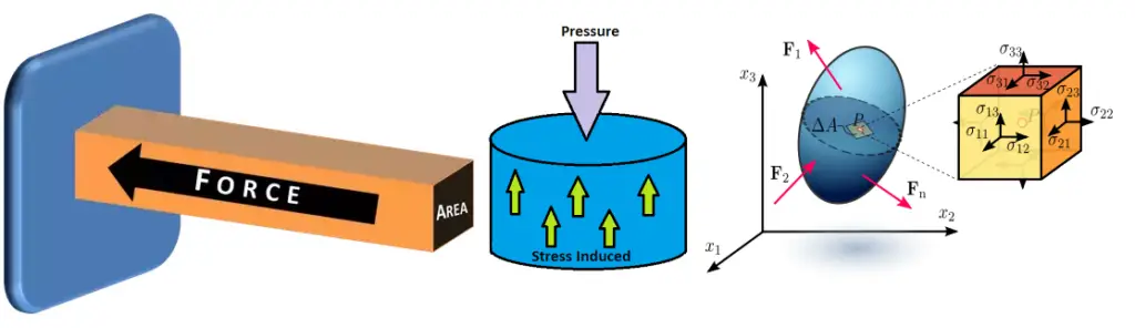
Pressure is an intrinsic property and most of the time related to fluids. It depends on the momentum transfer between the atoms of a liquid or gas volume (molecules constrained inside the volume) on a micro-scale.
While Stress is a consequence of the tendency of a body undergoing arbitrary deformation to spring back to its own reference state; To simplify stress is generated whenever a force is applied to a body to deform it.
In this article, I will list down the major differences between Pressure and Stress in a Tabular format.
Pressure vs Stress
Difference Between Pressure and Stress
Sr. No
Pressure
Stress
1
Pressure can be defined as the intensity of external forces acting at a point. It is the amount of external force applied per unit area. The pressure is exerted on the body.
Stress can be defined as the intensity of internal resistance force that is developed at a point due to the application of force or pressure. It is the amount of internal force being exerted per unit area. Stress is produced inside the material body.
2
Pressure is a unique property of thermodynamics or physics.
Stress is a material property.
3
Pressure always acts normal to the surface on which it acts.
The stress can be in any direction and any angle depending on the application of force.
4
Pressure always tries to compress the surface on which it is applied.
Stress can be tensile or compressive depending on the load type.
5
Pressure can be exerted on both liquids and gases.
Stress can only be exerted on solid materials.
6
Pressure is physically measured (measurable quantity) using pressure gauges, barometers, manometers, and other pressure-measuring devices or instruments.
Pressure is a positive unit and can be represented as “p”= F/A (F positive as direct force)
Stress can be either a positive or a negative force, this can be represented as Stress “Ϭ”= – F/A. (-F as internal resisting force)
8
The pressure is independent of the area of the contact surface. It remains constant and does not vary with changes in surface area. For example, Assume a 500 Pa pressure is applied to a 100 m2 area. Now even if you change the area to 10 m2 the pressure will remain constant. However, the calculated force will vary depending on the area.
On the other hand, stress varies with changes in surface area. Here, Force remains constant but an increase in the area causes the stress to reduce and vice versa. The magnitude of Stress varies inversely with the surface area on which it applies.
9
The pressure is a scalar field variable and does not depend on the direction as it always acts normal to the surface. The magnitude of the pressure at a point in all directions remains the same.
Stress is a vector variable and depends on the direction of the applied force. The magnitude of stress at a point in a different direction is different.
10
Pressure is the cause of stress
Stress is the result of pressure.
11
Pressure is a thermodynamic property.
Stress is a material property.
Table showing the Differences Between Pressure and Stress
Storage tanks are the containers/vessels which are used for storing the fluid. A group of tanks together is called ’Tank Farms’. The preferred design standard for Atmospheric storage tanks is API 650. The use of tanks is common in all kinds of plants. However, Petroleum and Water industries are the largest users of tanks.
Storage tanks are manufactured in different shapes, sizes, and capacities. Cylindrical tanks are the most common ones. Spherical tanks are used for storing LPG. Proper arrangement of tanks and pipes is required to optimize space and cost. Broadly, Storage tanks are used to
store feed products prior to processing.
hold partially processed products before further processing.
collect and hold finished products prior to delivery to market.
A) Process Plant
Refineries
Petrochemicals
Specialty chemicals
B) Terminals
Types of Tanks in Process plant
Based on the type of products to be stored, shapes, sizes, and potential to fire storage tanks can be grouped into various types like
Cone roof tanks: Low-pressure tanks for storing petroleum, water, food products, chemicals, and petrochemical products.
Floating roof tanks: The roof floats depending on the volume of stored products. Mostly used in oil refineries, such types of tanks reduce fire hazards.
Low-temperature storage tanks: Usually store cryogenic fluids line liquefied ammonia, propane, methane, etc.
Horizontal pressure tanks or Bullet tanks: Elliptical or hemispherical high-pressure tanks.
Hortonsphere pressure tanks: Store large quantities of fluids under pressure.
Underground Tanks for drain collection of the plant at atmospheric pressure.
FRP Tanks for corrosive fluids at atmospheric pressure.
The design of the tank farm and tank farm piping layout should take into consideration the following guidelines
Local rules and regulations.
Client specifications.
Maintenance and operation requirements.
OISD 118, 117, 117
NFPA 30
API 2030, etc.
Tank Farm Layout Consideration
The main considerations for tank farm layout are
The storage tanks shall be located at a lower elevation, wherever possible.
The storage tanks should be located downwind of process units.
All process units and diked (diked) enclosures of storage tanks shall be planned in separate blocks with roads all around for access and safety.
Provide a minimum of two-way access to enter the storage tank area. Preferably roads shall be provided all around the dike. Also, vehicular access is to be provided inside the dike for maintenance purposes.
Due to the risk of failure of storage tanks, an Earthen / RCC Wall(Dike) must be provided around the tank in order to hold the liquid.
A staircase shall be provided to enter in storage tank area from the outside dike.
The tank farm should be secured by fencing & access gates shall be provided.
Relative location for Area Layout
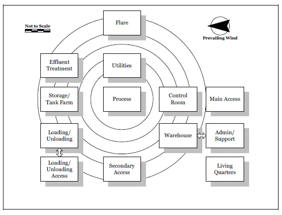
Fig. 2: Relative Location of Storage Tank Farm
Tank Farm Layout (Dike Enclosures)
Tanks shall be arranged in a maximum of two rows. Tanks having 47,700 cu.m capacity and above shall be laid in a single row.
The minimum distance between the tank shell and the inside toe of the dike wall shall not be less than half the height of the tank.
The Dike enclosure for the petroleum class shall be able to contain the complete contents of the largest tank in the dike.
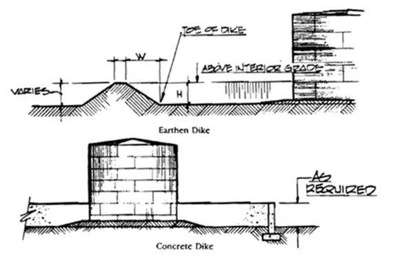
Width of Dike(W): Minimum 0.6m (Earthen dike); No specific (RCC dike)
The separation distance between the nearest tanks located in separate dikes shall not be less than the diameter of the larger of the two tanks or 30 meters, whichever is more.
In a diked enclosure where more than one tank is located, the intermediate dike is provided. The height of the intermediate dike wall should be 450 mm if concrete and 600 mm if earthen.
For locating tanks with respect to other tanks & equipment or vice versa, Refer to the minimum separation distance as mentioned in the company standard.
The optimum tank piping arrangement in a tank farm is the most direct route between two points allowing for normal line expansion and stresses. Usually, the following guidelines are followed while designing tank piping layout:
Piping located in a diked enclosure should not pass through any other diked enclosure directly.
The number of piping in the tank dike shall be kept minimum and routed directly outside the dike to Sleeper/Pipe rack.
Pumps and associated piping shall be located outside the dike wall.
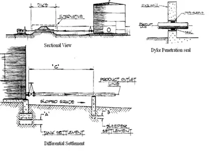
A pipe may only be routed through bund walls if it cannot be passed over the Dike walls (eg. Suction line). Pipe passing through the dike shall be sleeved and sealed.
Access platforms shall be provided for valve operation & for the instrument.
The pump shall be provided in a curbed area with proper provision for draining.
No piping shall be routed in the dropout(Maintenance)area.
The tank outlet line to the Pump suction nozzle is a gravity flow line. Pump suction piping from the tank shall be as short as possible.
Analyze the pipelines connected to the tank as per stress criteria given on a stress analysis basis.
Blanket gas(Fuel gas) & Vent gas line (Big bore size) can be routed & supported over the tank roof. Support location & load of such lines shall be marked in the tank vendor drawing. So the vendor will take care load for the design of the raft and will provide support cleat at the required location. Again need to discuss with the vendor for the high load if any.
Supporting Tank Piping
In general, the following rules can be considered for supporting pipes connected to storage tanks:
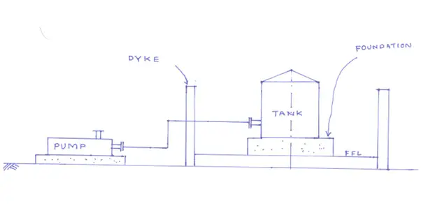
The tank Inlet & Outlet line can be supported either from the tank shell or the Tank foundation. If the support is taken from the tank foundation, this information shall be sent to the Civil department during the initial stage of the project & to the Tank vendor for providing vessel cleat.
Spring support or a Teflon pad may be introduced as the first support from the tank as per stress analysis based on tank settlement.
Keep the first support from the tank as far as possible. Group the lines for combined support.
Tank Farm & Piping
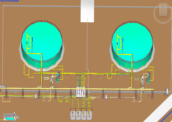
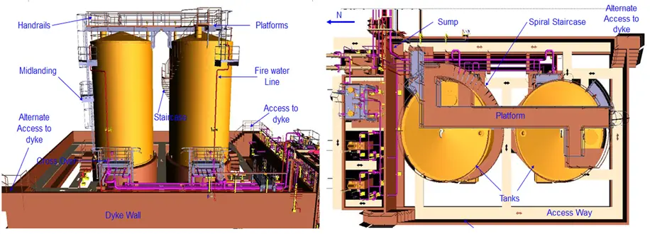
Fig. 6: Typical Tank piping arrangement inside dike wall
A fire in one part/section of the plant can endanger another section of the plant.
If a fire breaks out, it must be controlled/extinguished as quickly as possible to minimize the loss of life and property and to prevent the further spread of fire.
Foam systems & water spray systems are often provided as part of the fire protection system.
Permanent fire hydrants and monitors alternatively are used.
Locate hydrant & monitor along the road for easy access and for operation.
Online Course on Tank Farm Piping Layout and Stress Analysis
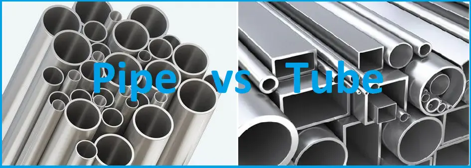
Pipes are used for transporting fluids and gases in Chemical, Petrochemical, Power Plants, Refineries, Storage units, Compressed air systems, Plumbing systems, etc. They are circular in cross-section and specified by Nominal Pipe Size.
What is a Tube?
Tubes are used for mechanical applications (Heat Exchanger, Fired heater, Boiler, etc.), for instrumentation systems (used for measuring instruments); for structural applications, etc and could be rigid or flexible. They are specified by their outer diameter and tube wall thickness, in inches or in millimeters.
Differences between Pipe and Tube
From a layman’s viewpoint, Both Pipe and Tube seem to be the same as they have many similarities like both are hollow, usually made from metals, can transfer fluids, etc. Many a time, these terms are used interchangeably. But in actual practice Tubes and Pipes are not the same as both possess different features. Through this article, we will try to investigate all such characteristics based on a few parameters like Size, Shape, Diameter, Thickness, Use, Availability, End Connection, Design Standard, etc.
Sr No
Parameter
Pipe Characteristics
Tube Characteristics
1
Shape
Pipes are always cylindrical or round in shape
Tubes are usually cylindrical in shape. However, tubes of different other shapes like square, rectangular, etc. are available.
2
Size
A pipe is Specified by Nominal Pipe Size (NPS) or Nominal Bore (NB).
The size of the Tubes is specified in millimeters or in inches by outside diameter.
3
Diameter
The outside diameter of pipe up to size 12” is numerically larger than the corresponding pipe size
The outside diameter of tubes is numerically equal to the corresponding size.
4
Thickness
Pipe Wall thickness is expressed in schedule numbers that can be converted into mm or inches.
Tube Wall thickness is expressed in millimeters, inches, or BWG (Birmingham wire gauge.)
5
Thickness Increment
Pipe thickness depends on the schedule, so there is no fixed increment
The thickness of tubes increases in standard increments such as 1 mm or 2 mm
Pipe vs Tube
Difference Between Pipe and Tube
Sr No
Parameter
Pipe Characteristics
Tube Characteristics
6
Application
Pipes are extensively used in all Process, Power & Utility lines to carry fluids.
Tubes are used in tracing lines, tubes for heat exchangers & fired heaters & instrument connections. They are more prevalent in the medical area, construction, structural, or load bearing.
7
Availability
Pipes are available as the small bore and the big bore
Normally small-bore tube is used in process piping. For structural use, tubes are available in custom sizes.
8
Structural Rigidity
Pipes are always rigid and resistant to bending
Tubes are available as rigid as well as flexible depending on the application. Rigid tubes are normally used in structural applications whereas copper and brass tubes can be flexible.
9
Joining and Stability
Joining pipes is more labor intensive as it requires flanges, welding, threading, etc.
Tubes can be joined quickly and easily with flaring, brazing, or couplings, but for this reason, they don’t offer the same stability
10
Tolerance
Pipe tolerances are not too restrictive.
Tolerances are very strict with tubes compared to pipes and tubes are often more expensive to produce than pipes
Pipes used in operating process plant
Sr No
Parameter
Pipe Characteristics
Tube Characteristics
11
Manufacturing
Pipe manufacturing is easier as compared to tubes
Tubes need more cumbersome tests, inspection, and quality control than pipes.
12
Cost
Cheaper
Costlier
13
Packing & Delivery
Delivered in the bundle as a bulk item. Delivery time is short.
Tubes are usually wrapped with a wooden box or thin film and delivered with much care. Delivery time is longer.
14
Production Quantity
Pipes are produced in mass quantity and for long-distance applications.
Tubes are produced in small quantities depending on requirements.
Tubes used inside a Fired Heater
Sr No
Parameters
Pipe Characteristics
Tube Characteristics
15
End Connection
The end connection of pipes is normally plain or beveled for welding purposes
Tubes are available with coupling ends, irregular ends, special screw thread, etc.
16
Surface Finish
The inner and Outer surface of the pipe is rough in comparison to the tube
Tubes are manufactured on both the inner and outer surfaces as smooth