Slug flow is a phenomenon that occurs in multiphase flow systems, particularly in pipes and pipelines carrying gas and liquid phases. It is characterized by the intermittent presence of large, cohesive bubbles or slugs of gas that travel through the liquid. This type of flow can lead to significant operational challenges, making slug flow analysis crucial for engineers and operators in industries such as oil and gas, chemical processing, and water treatment.
The purpose of this article is to explain the slug flow in piping and the static analysis of the piping system having slug flow using Caesar II. One of the major causes of piping vibration in operating plants is slug flow. So, it’s always preferable to design systems to overcome the effects of slug forces.
What is Slug Flow?
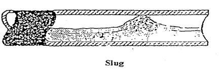
Slug Flow is a typical two-phase flow where a wave is picked up periodically by the rapidly moving gas to form a frothy slug, which passes along the pipe at a greater velocity than the average liquid velocity.
In this type of flow, slugs can cause severe and, in some cases, dangerous vibrations in piping systems because of the impact of the high-velocity slugs against fittings such as bends, tees, etc.
Characteristics of Slug Flow
Intermittency: Slug flow is marked by intermittent movement of gas bubbles within the liquid. These bubbles can merge to form larger slugs, causing a non-uniform flow.
High-Pressure Fluctuations: The movement of slugs can lead to pressure surges within the pipeline, which may damage equipment and create safety hazards.
Liquid Hold-up: During slug flow, there is a significant amount of liquid held up in the pipeline, which can impact the overall efficiency of the transport system.
Flow Regime Transitions: Slug flow can transition into other flow regimes, such as annular or stratified flow, depending on changes in flow rates or other conditions.
Is Slug Flow Dangerous?
Slug flows generate dynamic fluid forces, which may induce structural vibration.
Slug Flow
Excessive vibration may lead to component failures due to fatigue or resonance. Other reasons for worrying about Slug Flow are
the liquid trapped in the pipeline in low spots due to imbalances in the distribution of gas and liquid phases.
a flow rate change.
pipe geometry change
Pigging
significant density differences, etc
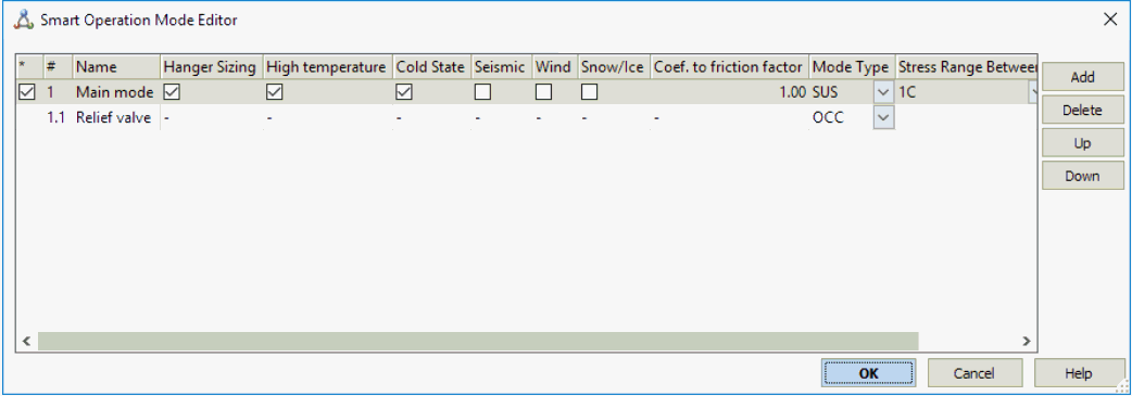
Such vibration problems may be avoided by thorough analysis, preferably at the design stage. Two types of Analysis Methods are prevalent in piping design-
Process Engineers will Analyze the two-phase flow regimes and inform accurately whether the given fluid can cause slug flow while flowing through the piping system. On a broad scale normally following lines are believed to give slug tendency.
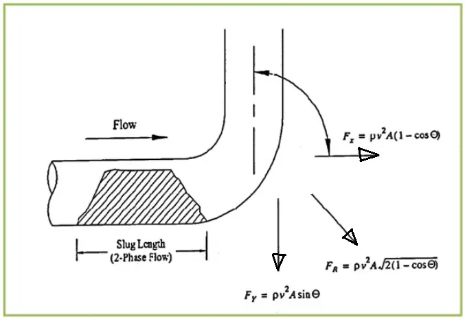
Slug force is equal to the change in momentum with respect to time. The equation used for the calculation of slug forces is provided in the attached figure:
Diagram Showing Applications of Slug Force
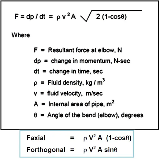
Use the following equations to calculate the Slug Force.
Multiply the calculated value with a suitable DLF. Normally a DLF of 2.0 is common to use.
Diagram Showing Slug Force Equation
From the above slug force calculation equation it is quite clear that:
The value of slug force will increase with an increase in fluid density
The slug force is directly proportional to pipe size; with an increase in pipe size, the resultant slug force will increase.
The calculated slug force is directly proportional to fluid velocity, which means with an increase in fluid velocity the impact of slug force will increase.
Also, the magnitude of slug force is directly proportional to the momentum flux (Rho X A X V2)
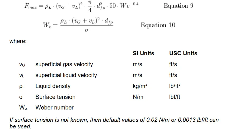
Alternate Equation for Slug Force Calculation
Alternatively, you can use the following slug force calculation equation as provided in Shell DEP 31.38.01.25, Feb 2023. As per clause 2.2.7, point no. 7 of the mentioned DEPs,
Slug flow piping system shall be designed to accommodate the reaction forces and vibration fatigue. The maximum reaction force Fmax shall be calculated in accordance with Equations 9 and 10.
Slug Force Calculation Formula as per DEP
Static Analysis of Piping Systems Carrying Slug Flow
Inputs Required for Static Slug Flow Analysis
Stress isometrics of the complete system.
Line parameters such as line temperatures, pressures, fluid density, pipe material, corrosion allowance, insulation thickness, density, etc.
Parameters required for Slug force calculation like slug density or liquid density, two-phase velocity, etc.
While performing slug flow analysis the following two assumptions are made
It is assumed that the slug is formed across the full cross-section of the pipe for maximum impact. This configuration is least probable for vertically down word flow as no hold–up is possible for the accumulation of liquid and eventual formation of the slug. Hence slug force at elbows for vertically downward flow lines is not considered.
It is assumed that the reader knows the normal static analysis of the piping system using Caesar II.
Sample Case Study for Slug Flow Analysis in Caesar II
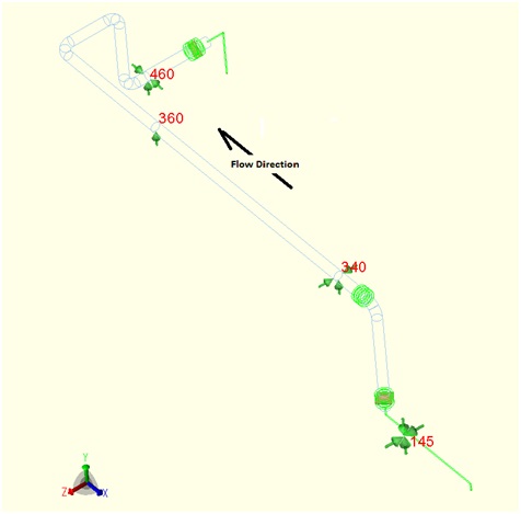
Let’s assume the shown system is subjected to slug flow. The parameters for the pipe are as mentioned below:
Pipe: A106B, 6”, Sch 40
CA=3 mm
T1=100 degree C
T2=75 degree C
P1=15 bar
Liquid Density=950 Kg/m^3
Two-phase Velocity=10.53 m/s
Stress System under consideration
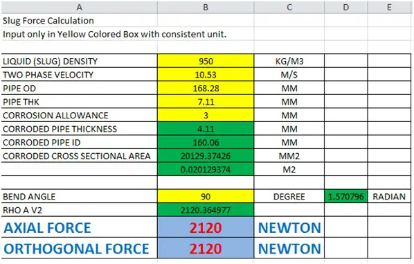
After modeling the piping system following the conventional method, we have to calculate the slug force and apply the same to the system. Normally all organizations have their Excel spreadsheet to calculate Slug Force. A typical Excel spreadsheet for slug force calculation is shown in the below-attached figure for your reference.
Excel Spreadsheet for Slug force calculation
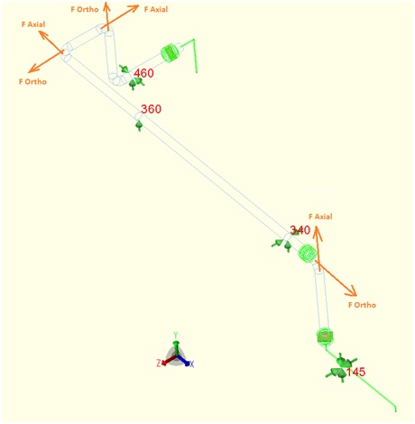
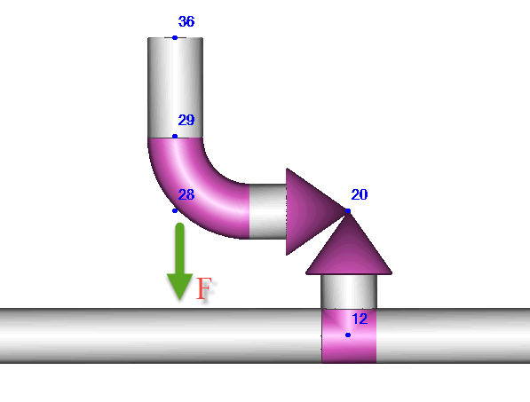
So if we use a DLF of 2 then each axial and orthogonal force will be 4240 N. We have to incorporate this force in the Caesar II input spreadsheet. Check the below-mentioned figure for the direction of forces.
Slug force in Bends with Application direction
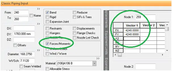
Now we will input the axial and orthogonal forces at all changes in direction as shown in the attached figure.
To enter forces click on the Forces button in the Caesar II spreadsheet.
Provide the node number and magnitude of forces with the proper direction.
Similarly input forces in all bends (other than vertically downward bends).
Caesar Spreadsheet Showing input methodology of Slug Force
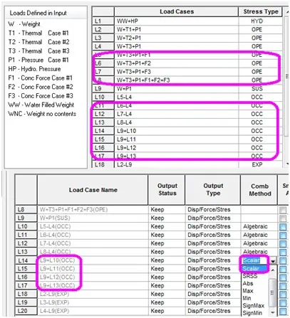
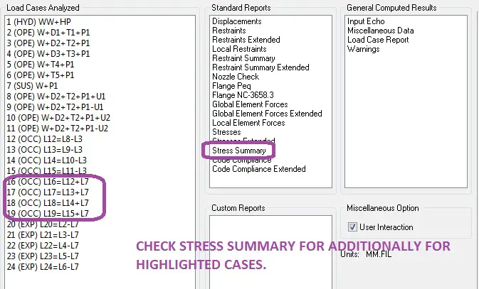
The next step is to prepare the required load cases. Some additional load cases need to be prepared for static analysis of slug force. The same is shown in the figure below.
Caesar II Load cases for Slug Flow Analysis
Prepare the load cases as mentioned in the figure.
Make stress types occasional
Use combination methods such as Scalar
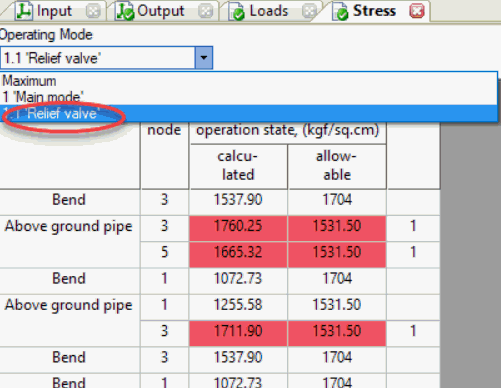
Understanding the Slug Flow Analysis Output
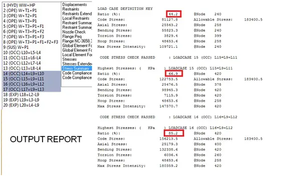
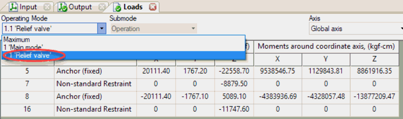
Additionally, We have to check code compliance for load cases L14 to L17 and ensure that the values are well within code allowable values.
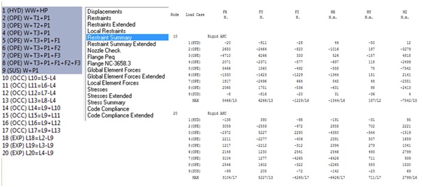
We have to check forces and displacements for load cases L1 to L9.
Refer to the below-mentioned figures for reference:
Caesar II Code compliance check report
Caesar II Restraint Summary check report
Keep all stresses, forces, and displacements within the allowable limit. If exceeds then try iteration with the support location change, support type change, or pipe routing change.
Slug Flow Prevention/ Mitigation
To effectively mitigate the risks associated with slug flow, a variety of preventive measures can be adopted. Here are some essential strategies for prevention:
1. Optimized Pipe Configuration
Designing the piping layout to minimize the potential for liquid accumulation is crucial. This includes avoiding configurations that create pockets where liquids can be collected. A well-thought-out design can significantly reduce the likelihood of slug formation.
2. Low Point Drains and Traps
Incorporating low-point drains, traps, or bypasses in the pipeline is an effective way to prevent liquid accumulation. These features allow any trapped liquid to be removed, maintaining a more consistent flow and reducing the chance of slugs developing.
3. Regular Insulation Checks
Periodic inspections of insulation can help minimize condensate formation, which can contribute to slug flow. Ensuring that insulation is intact and effective reduces the risk of excess liquid buildup in the system.
4. Complete Draining Design
Piping and equipment should be designed to allow for complete drainage. This design consideration eliminates pockets where liquid can become trapped, further preventing slug flow.
5. Maintenance of Traps and Valves
Including traps, pressure control valves, safety valves, and rupture disks in your preventive maintenance program is vital. Regular checks on these components ensure they function correctly and help manage flow conditions effectively.
6. Review of Abandoned Equipment
Conducting a review of any abandoned equipment and piping systems can identify potential sources of liquid buildup. Addressing these areas can help prevent slugs from forming in the active portions of the system.
7. Thoughtful Material Selection
Choosing materials with adequate tensile strength is important for withstanding dynamic transients and impact loads. For example, avoiding brittle materials like cast iron can prevent structural failures due to slug impacts.
8. Proper Support Design
Ensuring that supports are designed to accommodate transient performance is essential. This consideration helps maintain the integrity of the piping system during fluctuations in flow.
9. Use of Slug Catchers
Integrating slug catchers at the pipeline outlet can effectively manage and collect slugs. These devices help minimize the impact of slugs on downstream equipment and maintain a more stable flow.
Slug Flow is a typical two-phase flow where a wave is picked up periodically by the rapidly moving gas to form a frothy slug, which passes along the pipe at a greater velocity than the average liquid velocity. slugs can cause severe and dangerous vibrations in piping systems because of the impact of the high-velocity slugs against fittings such as bend, Tee, etc and it can cause the failure of the piping system.
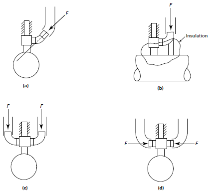
What is Slug Force?
Slug Force is equal to the change in momentum with respect to time, i.e, Force F=dp/dt. The equation of slug force for a piping elbow is given by:
What are the lines that are prone to Slug Flow?
Process Engineers will Analyze the two-phase flow regimes and inform accurately whether the given fluid can cause slug flow while flowing through the piping system. On a broad scale normally following lines are believed to gave slug tendency. 1. Vacuum Transfer Lines 2. Condenser Outlet Lines 3. Re-boiler Return Lines 4. Fired Heater outlets 5. Boiler Blow down lines. 6. Various Pipeline Flowlines (Process Discipline to Confirm case by case)
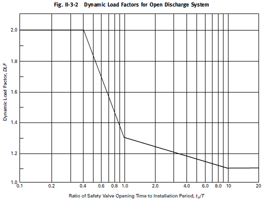
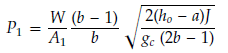
There’s two methods to estimate the dynamic equivalent thrust force F:
ASME B31.1 method
Direct calculation of V1 и P1 by special software like Hydrosystem
ASME B31.1 Method
Equivalent dynamic thrust force can be estimated by the equation: F = DLF ∙ F1
where DLF – dynamic load factor, depending on the first natural period of piping. If the period is unknown the DLF=2.0.
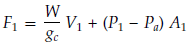
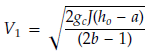
F1 – static reaction force, kgf. May be computed by the following equation:
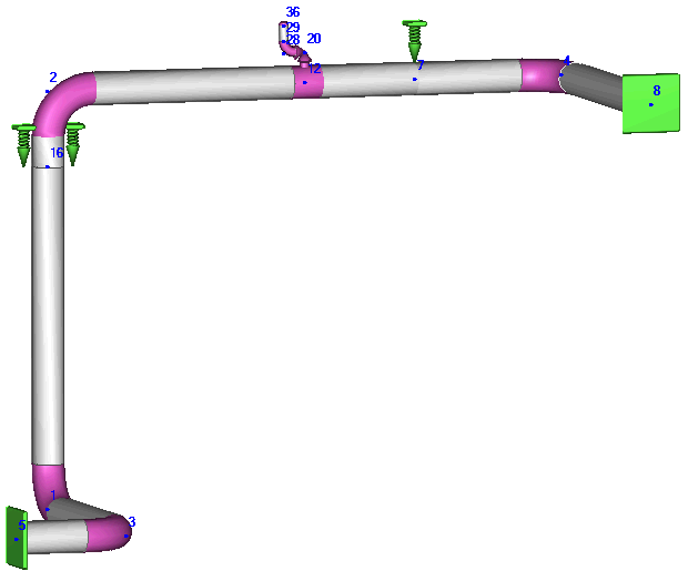
where W – mass flow rate (relieving capacity stamped on the valve by 1.11), kg/sec gc=9.81 m/sec² – gravitational constant, Pa – atmospheric pressure, kgf/sm² A1 – exit flow area, sm² A1=p∙(D-2t)²/4 V1 – exit velocity (node 36), m/sec
P1 – static pressure, kgf/sm²
h0 – stagnation enthalpy at the safety valve inlet, MJ/kg
J = 101970.408 m*kgf/MJ
a, b – constants according to the table below
Columns or Towers, used for distilling raw materials (Crude Oils) are very important equipment in any process industry. Every process piping industry must have several columns. Lines of various diameters and properties (Process Parameters) are connected to Columns at different elevations. Stress analysis of all large bore lines connected to the column is required to assess proper supporting and nozzle loading. Looking at the construction of the column, it has a number of trays at different elevations. The temperature at each tray location differs based on the process. In the following article, I will try to explain the methodology followed for stress analysis of Column Piping using Caesar II.
Stress analysis of Column Piping will be discussed in the following points:
The following data are required while modeling and analyzing column connected lines:
a) Column G.A.drawing with all dimensions, nozzle orientation, materials, etc. b) Column temperature profile. c) Line Designation Table/ Line list/Line Parameters and P&ID. d) Column line isometrics. e) The allowable nozzle load table as specified in Project Specification.
2. Temperature profile for Column/Tower
Various organizations use different methods for creating a column temperature profile. Here I will describe two methods that are most widely used.
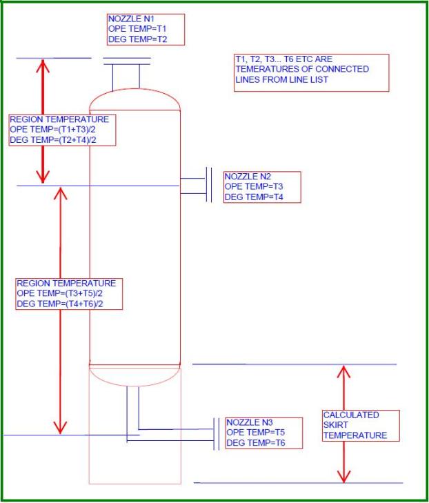
Temperature profiles for towers are normally created based on connected outlet lines. So in the P&ID mark the big size (big size means nozzle size which will make a considerable impact in temperature change) column outlet nozzles. Then write down the operating and design temperatures beside those lines from the line list. Let’s assume that there are three big sizes (N1, N2, and N3 as shown in Fig. 1) outlet nozzles in a typical tower. So temperature profile for that column can be created as shown in Fig. 1. This method is the most widely used method among prevailing EPC industries.
Fig. 1: Temperature profile creation for a typical tower- Method 1
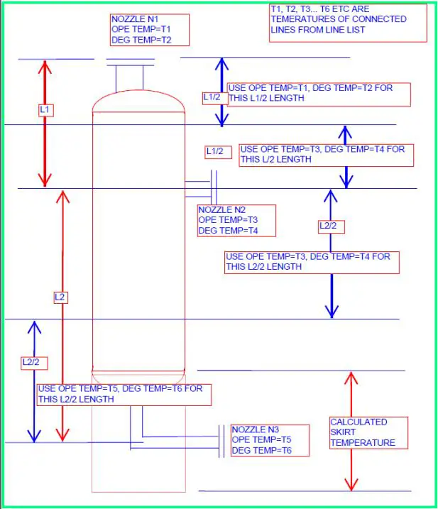
Again the temperature profile of the above tower can be generated using the method mentioned in Fig. 2. Many of organizations use this method too.
Fig. 2: Temperature profile Creation for a typical Column -Method 2
Few organizations use the operating and design temperatures mentioned in equipment GA as the equipment operating and design temperature. However, the above two methods mentioned will result in thermal growth close to reality.
3. Modeling the Column/Tower in Caesar II
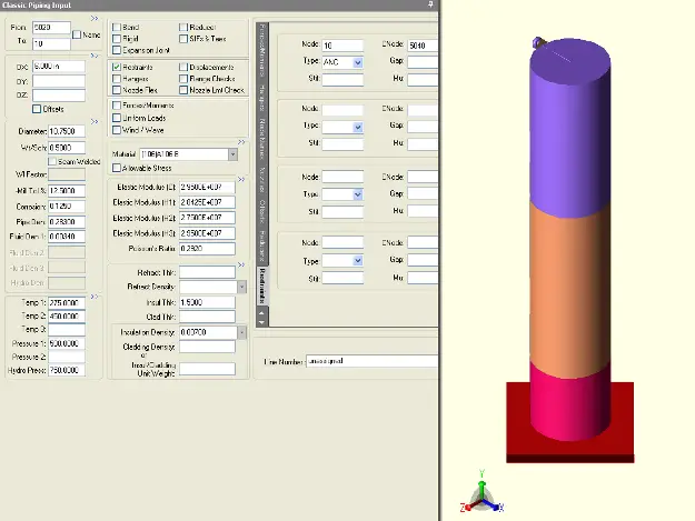
All equipment modeling is almost similar. Start modeling the tower from the skirt and go up or start from the nozzle of interest and go down till the skirt as per your choice. It is a better practice to use node numbers in such a way that the equipment nodes can easily be separated from the piping nodes. I personally model equipment starting from node 5000.
Let’s start with a typical nozzle flange. So model 5000-5020 is a nozzle flange with nozzle diameter and thickness as mentioned in the equipment GA drawing. Sometimes, Vendor-GA may not be available (during the initial phase of the project), so in such situations use engineering drawing as the basis for modeling. Normally mechanical departments have a minimum nozzle thickness chart based on flange rating and corrosion allowance. Take nozzle thickness from that chart or otherwise assume nozzle thickness as two sizes higher than the connected pipe thickness. Use temperatures as mentioned in the above two diagrams (Fig. 1 or Fig. 2) from flange onwards, pressure, corrosion allowance, materials, insulation thickness, density, etc as mentioned in the reference equipment drawing.
Then, model 5020 to 10 as pipe elements with length from reference drawing (Normally nozzle projection from equipment centreline is provided, in that case, calculate the nozzle length by subtracting the equipment outside radius and flange length already modeled). Provide Anchor at node 10 with C-node at 5040. Providing node numbers for nozzles as 10, 20, etc will put all these nodes at initial nodes in restraint summary which helps me in checking nozzle loads very quickly. You can provide separate nodes if you wish. This completes the nozzle model. Now we will model the equipment.
Model 5040 to 5060 as a rigid body with zero weight with length=half of equipment OD, material as provided in reference drawing, temperature as mentioned in the above figures, pressure, and other parameters from reference equipment drawing. This element will take you to the center of the equipment. From this part onwards simply model the equipment as pipe elements taking temperature profile as mentioned in the above figures. Check the diameter and thickness in the reference drawing as those values sometimes change as you proceed from the top toward the skirt. Finally model the skirt as a pipe element with temperatures calculated as mentioned in the last paragraph of this topic and pressures, fluid density, and corrosion allowance as zero. Provide a fixed anchor at bottom of the skirt. Refer to Fig. 3 for a sample model of the column. Different colors are for different temperatures.
Fig. 3: A simple model of a Tower in Caesar II
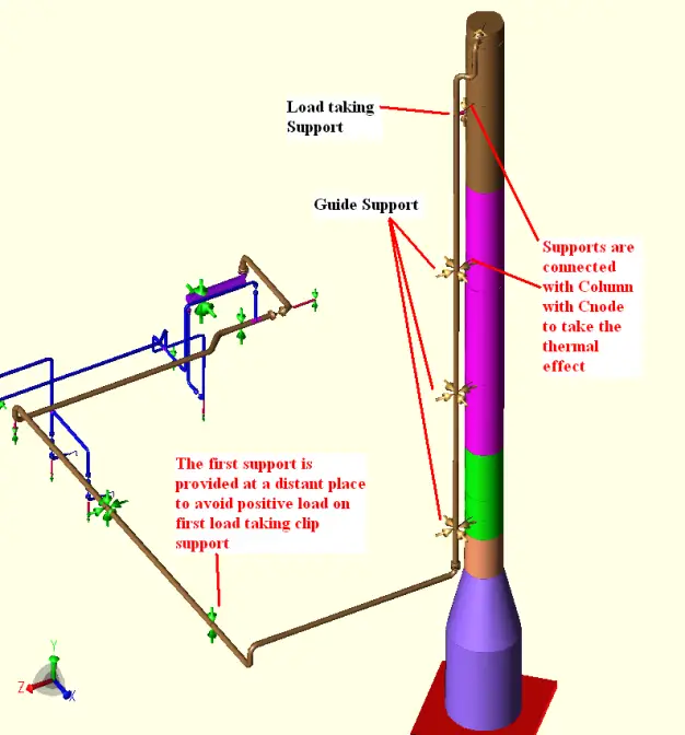
4. Supporting of Column Connected Piping System
The pipes are normally supported by the column itself. This type of support is called cleat support or clip support. The first support from the column nozzle is a load-taking support that carries the total vertical load of the pipe. Try to place this load-taking support as near the nozzle as possible. Rest all are guide supports.
As the clips are connected to the tower body we have to model clips from the column and connect the supports with a C-node to take the thermal effect of that location. The load-bearing capacity of the clip supports is normally standardized by pipe support standards. So sometimes it may appear that the load at first load-taking support is exceeding the clip load bearing capability (This could happen if a very large size line is connected towards the top of the column, overhead lines). In those cases, we have to take 2nd support from the nozzle as a load-taking support as well.
This support has to be a Spring hanger support which will share part of the load of the first load taking the support. From that point onwards guide supports will be used based on the standard guide span as specified in the project specification. A sample Caesar II model is shown in Fig 4 for your reference to explain the clip supports. Model the clip as a rigid body with zero weight with equipment properties when inside equipment and with ambient temperature when outside equipment.
Fig. 4: Caesar II model showing Clip/Cleat Supporting
5. Nozzle Load Qualification
Allowable nozzle loads are normally provided by equipment vendors and mentioned in general arrangement drawings. Few organizations have a standard load table based on nozzle diameter and flange rating. So compare your calculated loads at the nozzle anchor point with these allowable values to find if calculated loads are acceptable or not. If loads are exceeding the allowable values modify the supporting or routing to reduce your nozzle loads. In some situations when routing change is not feasible perform WRC 537/297 or perform finite element analysis (FEA- Nozzle Pro) to check whether generated stresses are acceptable. In extreme cases send your nozzle loads to the vendor for their acceptance.
Skirt Temperature Calculation
Calculate skirt temperature following the given equation:
Average Skirt Temperature=(T-Ta)*F+ Ta; in degree centigrade
Here Ta=Ambient Temperature in degree Centigrade; T=Temperature at the top of the skirt; F=[83.6/{(K*h/t^0.5)+15.5}]; K=insulation constant=1.0 for fire brick insulation=1.6 for non-insulated; h and t are skirt height and thickness respectively.
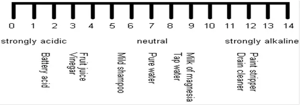
A pH Analyzer or pH meter is an electronic instrument that measures the pH value of a solution to measure acidity or alkalinity. pH can be measured and its value ranges between 0 and 14. Solutions with a pH<7 are acidic, whereas those with a pH>7 are alkaline. In “pH”, the term “p,” denotes the mathematical symbol for negative logarithm, and “H,” is the chemical symbol for Hydrogen. So, A pH meter or pH Analyzer analyzes the solution to measure the hydrogen ion activity in the solution.
A pH analyzer is an important instrument in many industrial and laboratory applications because it measures the acidity or basicity of a solution by determining the concentration of hydrogen ions (H+) in the solution. The pH value of a solution can range from 0 to 14, with 7 being neutral, values below 7 indicating acidity, and values above 7 indicating basicity.
Here are some reasons why pH analyzers are important:
Quality control: In many industrial processes, the pH of a solution is a critical parameter that needs to be monitored to ensure product quality and consistency. For example, in the manufacturing of chemicals, pharmaceuticals, food, and beverages, the pH of a solution can affect the reaction rate, product yield, and sensory characteristics of the final product.
Process optimization: By monitoring the pH of a solution in real time, pH analyzers can help operators adjust process variables such as temperature, pressure, and chemical dosing to optimize the process and improve efficiency.
Environmental monitoring: In environmental monitoring applications, pH analyzers are used to measure the pH of water and wastewater to ensure compliance with environmental regulations and to monitor the health of aquatic ecosystems.
Safety: In some industrial processes, the pH of a solution can affect the safety of workers and equipment. For example, acids and bases can be corrosive to metal pipes and vessels, leading to leaks and equipment failure. By monitoring the pH of a solution, pH analyzers can help operators take corrective action to prevent accidents and ensure the safety of personnel and equipment.
Overall, pH analyzers are important instruments in many industrial and laboratory applications because they provide accurate and reliable measurements of pH, which is a critical parameter in many chemical and biological processes.
What is pH?
The concentration of the hydrogen ion in a solution is a measure of its acidity or basicity. This concentration is expressed in terms of the pH of the solution. ie: the negative logarithm of the hydrogen ion concentration.
pH = -log[H+]
Fig. 1: pH Scale
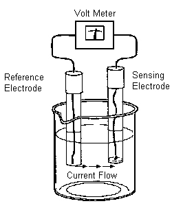
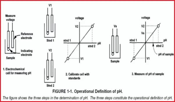
pH Measurement
Electrochemical cell: The cell consists of a sensing electrode whose potential is directly proportional to pH, a reference electrode whose potential is independent of pH and the liquid to be measured. The overall voltage of the cell depends on the pH of the sample.
Because different sensing electrodes have slightly different responses to pH, the measuring system must be calibrated before use.
The critical step in the operational definition of pH is calibration.
Fig. 2: pH Measurement
pH analyzer working principle
The system is calibrated by placing the electrodes in solutions of known pH and measuring the voltage of the cell. Cell voltage is a linear function of pH, so only two calibration points are needed.
The final step in the operational definition is to place the electrodes in the sample, measure the voltage, and determine the pH from the calibration data.
Fig. 3: Calibration Procedure
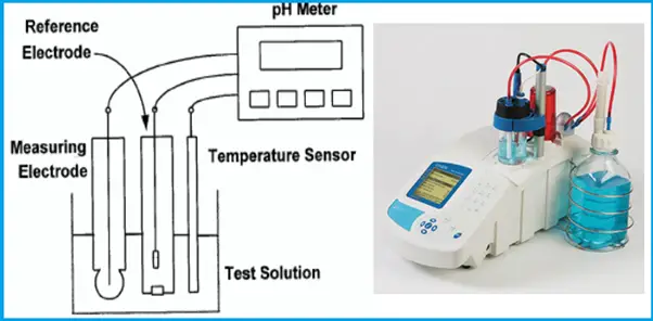
pH Meter
The cell consists of a measuring electrode, a reference electrode, a temperature-sensing element, and the liquid being measured. Refer to Fig. 4.
The voltage of the cell is directly proportional to the pH of the liquid.
The pH meter measures the voltage and uses a temperature-dependent factor to convert the voltage to pH.
Fig. 4: Typical pH Meter
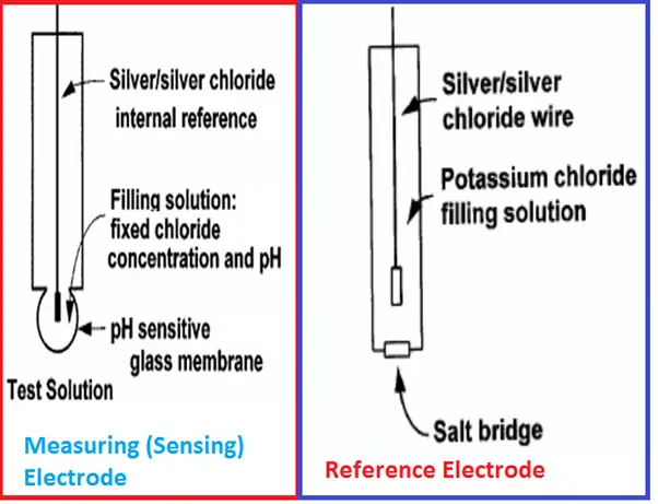
Measuring (Sensing) Electrode of pH Meter
The outside surface of the glass membrane contacts the liquid being measured, and the inside surface contacts the filling solution.
An electrical potential directly proportional to pH develops at each glass-liquid interface.
Because the pH of the filling solution is fixed, the potential at the inside surface is constant.
The overall potential of the measuring electrode equals the potential of the internal reference electrode plus the potentials at the glass membrane surfaces.
Because the potentials inside the electrode are constant, the overall electrode potential depends solely on the pH of the test solution.
The potential of the measuring electrode also depends on temperature. If the pH of the sample remains constant but the temperature changes, the electrode potential will change. Compensating for changes in glass electrode potential with temperature is an important part of the pH measurement.
Fig. 5: Electrodes
Reference Electrode of pH Analyzer
The reference electrode is a piece of silver wire plated with silver chloride in contact with a concentrated solution of potassium chloride held in a glass or plastic tube.
The fixed concentration of chloride inside the electrode keeps the potential constant.
A porous plug salt bridge at the bottom of the electrode permits electrical contact between the reference electrode and the test solution.
Temperature Compensation for pH Analyzers
Millivolt signals produced by the pH and reference electrodes are temperature-dependent.
However, the pH and reference electrode combination exhibits an iso-potential point, where the potential is constant with temperature changes.
This iso-potential point is designed to be at 7.0 pH and 0 mV.
Using the iso-potential point with theoretical knowledge of electrode behavior makes it possible to compensate (correct) the pH measurement at any temperature to a reference temperature (usually 25°C), using a temperature signal from the temperature element.
Converting Voltage to pH in pH meter
E(T) = E°(T) – 0.1984 T pH
E(T): Cell voltage at temperature T.
E°(T) is the sum of the following
The potential of the reference electrode inside the glass electrode.
The potential at the inside surface of the glass membrane.
The potential of the external reference electrode.
The liquid junction potential.
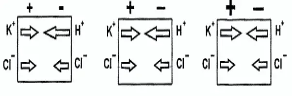
pH analyzer Liquid Junction Potential
The junction separates a solution of potassium chloride on the left from a solution of hydrochloric acid on the right. The solutions have equal molar concentrations.
Driven by concentration differences, hydrogen ions, and potassium ions diffuse in the directions shown. The length of each arrow indicates relative rates.
Because hydrogen ions move faster than potassium ions, the positive charge builds up on the left side of the section and the negative charge builds up on the right side.
The ever-increasing positive charge repels hydrogen and potassium ions. The ever-increasing negative charge attracts the ions.
Therefore, the migration rate of hydrogen decreases, and the migration rate of potassium increases. Eventually, the rates become equal.
Because the chloride concentrations are the same, chloride does not influence the charge separation or the liquid junction potential.
Fig. 6: Liquid Junction Potential
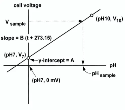
Buffers & Calibration
Fig. 7 shows the performance of an ideal cell: One in which the voltage is zero when the pH is 7, and the slope is -0.1984T over the entire pH range. In a real cell, the voltage at pH 7 is rarely zero, but it is usually between -30 mV and +30 mV. The slope is also seldom -0.1984T over the entire range of pH. However, over a range of two or three pH units, the slope is usually close to ideal.
Fig. 7: Cell performance curve
Because pH cells are not ideal, they must be calibrated before use. pH cells are calibrated with solutions having exactly known pH, called buffers.
pH Meter Sensor Installation
Immersion and insertion applications
If a pH sensor is to be inserted directly into a pipe, choose a location that is always flooded.
So long as a liquid film provides a conductive path between the glass membrane and the reference junction, the sensor will produce a reading. The reading, however, is the pH of the film, not the process liquid. If the film dries out, the sensor will appear to have failed.
Always consider the velocity and density of the liquid flowing past the sensor.
A dense liquid moving at a high flow rate can deform the sensor, particularly if it extends some distance into the stream.
Install pH sensors with the bulb down, within 80° from vertical.
The potassium chloride and buffer solution inside the glass electrode must completely wet the inside surface of the glass bulb, and there must be a conductive path between the internal reference electrode and the inside glass surface. Installing the electrode bulb pointed up or at an angle too close to the horizontal will break the connection.
pH sensors need regular calibration and, in some applications, regular cleaning.
The ease with which the sensor can be removed from the piping should always be considered.
Maintenance of pH Analyzer:
Maintenance of pH measurement systems involves mostly cleaning and calibrating the pH sensor. The analyzer itself requires almost no maintenance.
CLEANING pH SENSORS: The frequency at which a sensor should be inspected and cleaned can be determined only by experience. If the process liquid coats or fouls the sensor, frequent cleaning may be necessary. If the process does not contain a high level of suspended solids, the need for regular cleaning will be less.
CALIBRATING pH SENSORS: The frequency at which sensors should be calibrated can be determined only by experience.
However, many factors influence the calibration frequency are:
Sensors installed in dirty or corrosive process streams usually require more frequent calibration than sensors used in clean water.
Sensors measuring extreme pH values, particularly high pH, also require more frequent calibration than sensors measuring mid-range pH.
Noise pH readings in pH Meters
Noise is a rapid, random fluctuation in a signal. Noisy pH readings can have many causes.
The pH signal is high impedance, so it is susceptible to environmental noise. Problems with environmental noise can also be minimized by pre-amplifying the signal at the sensor.
The impedance of the glass electrode increases as temperature decreases. An increase in impedance caused by a cold sample might be contributing to the noise.
A plugged or depleted liquid junction can also be a source of noise.
Noisy readings, particularly if accompanied by offsets that disappear when the sample is electrically isolated from the process piping, can be a symptom of ground loops.
Noise can be a severe problem when measuring the pH of high-purity water. pH readings in high-purity water are also flow-sensitive. High flow can produce very noisy readings as well as offsets as great as 0.5 pH units. The problem is likely caused by variations in the electrical potential at the surface of the junction plug. The fluctuating potentials are related to the flow of filling solution through the junction pores.
Drift in pH Analyzers
Drift is a gradual increase or decrease in a signal not caused by an actual change in the process liquid.
Temperature changes can cause drift.
Dirty sensors often produce pH readings that drift.
The memory of past junction potentials can also lead to drift.
Ground Loops in pH meters
A ground loop exists when a circuit is connected to the earth’s ground at two or more points. Because the potential of the earth varies from point to point, two or more connections to the ground cause currents to flow. If the current flows through a signal-carrying wire, the result is a noisy, offset signal.
Procedure to check for ground loops
Remove the pH sensor from the process liquid.
Calibrate the sensor in buffers. Be sure there is no direct electrical connection between the container holding the buffer and the process liquid or piping.
Strip back the ends of the heavy gauge wire. Connect one end of the wire to the process piping or better, place it in the process liquid. Place the other end of the wire in the container with the buffer and sensor. The wire makes an electrical connection between the process and the sensor.
If the pH reading changes or becomes noisy after making the connection, a ground loop exists. If no symptoms develop a ground loop probably does not exist.
Recommendation for Accurate pH Measurement in pH Analyzers
Correct Electrode Storage: Correct electrode storage maximizes electrode performance and extends the electrode life. Do not store pH electrodes in distilled water. The filling solution will be diluted and the electrode response will be slow.
Proper Maintenance and Cleaning: Inspect the electrode weekly for scratches, cracks, or salt crystallization. If the readings become slow or drifty, clean the electrode per the manufacturer’s instructions. Excessive cleaning may impair electrode performance and shorten electrode life.
Stirring: Stir all buffers and samples at a uniform rate to obtain a representative sample measurement and improve electrode response time. Use a magnetic stirrer at a moderate speed. Use a piece of insulating material (e.g. Styrofoam or cardboard) between the stir plate and the beaker to prevent heat transfer.
Filling Solution Level: The filling solution level must be higher than the sample level to maintain a uniform flow of filling solution. At least 1 inch above sample height is recommended
Rinsing: Rinsing prevents contamination by carryover on the electrodes. Rinse with de-ionized water or an aliquot of the buffer, standard, or sample. Do not wipe the pH electrode glass bulb. Transfer of static charge onto the glass bulb will result in a slow or drifty response.
pH Buffers: pH Buffers should be accurate and free of contamination. Keep the buffer or standard bottle tightly sealed. Do not reuse buffers and standards. Verify the buffer or standard is within the expiration date before use. If trouble arises always use fresh buffers.
Temperature: To account for pH slope, buffer, and sample changes, use a separate or integrated automatic temperature compensation probe (ATC). Calibrate at least once a day with 2 or 3 buffers that bracket the expected sample range. Choose pH buffers that are no more than 3 pH units or no less than 1 pH unit apart.
Electrode Cleaning: After any of these cleaning procedures, drain and refill the reference chamber and soak the electrode in storage solution (or pH 7 buffer) for one hour.
General – Soak the electrode in 0.1M HCl or 0.1M HNO3 for half an hour.
A second general cleaning procedure involves soaking the electrode in a 1:10 dilution of household laundry bleach in a 0.1-0.5% liquid detergent solution in hot water with vigorous stirring for 15 minutes.
Removal of Deposits:
Protein- Soak the electrode in 1% pepsin in 0.1M HCl for 15 minutes.
Inorganic- Soak the electrode in 0.1M tetrasodium EDTA solution for 15 minutes.
Grease & Oil- Rinse the electrode with a mild detergent of methanol solution.
Applications of pH Analyzers/pH Meters
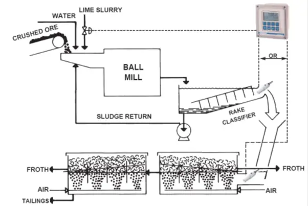
Copper Floatation Process (Fig. 8):
Crushed ore (containing 1 to 2% copper), along with water and a lime slurry, is fed into a ball mill.
This rotating drum contains steel balls that further crush the ore to a fine powder.
When the ore/lime slurry emerges from the mill, it is fed to a rake classifier.
Particles that are too large to pass from the classifier are returned to the mill, while the overflow is discharged to flotation cells.
Air is injected into the flotation cells, and foaming agents are added, creating a froth.
Copper ore particles, due to their relatively lightweight, become a part of this froth, while heavier particles, such as iron ore, do not.
The copper-rich froth, containing 20 to 40% copper, is then separated from the solution for further processing.
Fig. 8: Copper Floatation Process
Principle: As seen above, rich copper ore is separated from crude copper sulfide ore by means of a flotation process, that takes advantage of the physical (as opposed to chemical) properties of small copper ore particles. To maximize the yield of copper, pH control is necessary for the flotation tanks.
pH CONTROL:
The condition of the froth is directly dependent on pH.
The flow rate of lime slurry is therefore regulated to keep the pH within the acceptable range.
If pH is too low, iron will be entrapped as well as copper, decreasing the value of the copper ultimately recovered.
If too much lime is added, the result is a dilute froth that requires additional concentration in later stages, increasing the operating costs and wasting time.
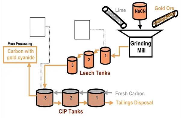
Gold Ore Processing Using Cyanide (Fig. 9):
The heap-leaching solution continuously flows over the ore and may be collected and stored in a pond.
In heap leaching, the carbon is usually held in a fixed column and the solution is passed over the columns repeatedly.
The gold cyanide is typically separated from the pregnant liquor using carbon adsorption beds.
The activated carbon adsorbs the gold cyanide complex on the surface of the carbon particles.
The gold cyanide in the pregnant solution is adsorbed on granular activated carbon inside the carbon in pulp (CIP) tanks.
Later, the carbon is washed with hot caustic to remove the gold and then rinsed with acid to regenerate the carbon particles for reuse.
The coarse-laden carbon particles are screened out of the last tank, and washed with caustic to remove the gold cyanide, and the gold metal is produced using a process called electrowinning.
Fig. 9: Schematic diagram of Gold Ore Processing Using Cyanide
When pregnant liquor contains large amounts of silver, and zinc, precipitation may be used instead of carbon adsorption.
Zinc precipitation liberates the gold metal by adding zinc metal to the solution, which rapidly displaces the gold in the Au(CN)2.
Once the solution has been depleted of the gold cyanide, it is called barren solution and is returned to the heap, to continue the leaching process.
Long-term use of the solution will cause the pH of the solution to change, so makeup caustic and/or lime may be added periodically to the barren solution. This process occurs so slowly that online instrumentation is rarely required.
Due to the rapid reactions taking place in an agitated leach process, automatic pH control is strongly recommended.
pH MEASUREMENT:
pH is controlled between 11 and 12 during the leaching process.
pH values below 11 favor the formation of HCN, hydrogen cyanide.
Hydrogen cyanide is a colorless and poisonous gas that, if released due to lower pH values, can quickly become deadly.
Cyanide is also a relatively expensive chemical, so small losses in heap leaching can amount to large makeup costs over time.
Gas leaks into the environment are a risk to the mine personnel and future liability to the mining corporation that can be avoided using pH measurement.
Boiler Flue Gas-Scrubbing System:
After fly ash removal, the flue gas is bubbled through the scrubber, and the slurry is added from above.
Water absorbs the SO2 gas which reacts to form sulfite ions. These ions can further react with dissolved oxygen to yield calcium sulfate.
The scrubbed gas may be heated, to prevent condensation, and then discharged in a stack.
Spent scrubbing liquids are sent to a clarifier, where much of the water is reused.
Spent solids are removed in a heavy slurry to a settling pond. The water (with makeup fresh water, as needed) is returned to the scrubber.
Both lime and limestone can be used to combine with the sulfite ions to form calcium sulfate (gypsum). Neither dissolves well in water and therefore, both are pumped in slurry form to the scrubber tower.
A pH sensor in a recirculating tank is used to control the feed of solid lime or limestone.
Lime slurry is more alkaline, having a pH of 12.5 while limestone slurry is roughly neutral. A lime-based system will therefore add more lime when the pH drops below 12 and a limestone-based system will be controlled around 7.
Unless one or the other is added, the SO2 gas will quickly drive the pH acidic. The calcium compounds produced in scrubbers tend to accumulate in recirculation loops and can cause a buildup of scale.
Scale on the spray nozzles affects the atomization of the water droplets and reduces the scrubbing efficiency. Scale on the return piping reduces the flow rate and changes the thermal balance of the system.
The tendency to scale is limited by additives such as chelating agents and phosphates, but these additives are generally only effective at higher pH levels.
pH control is necessary to forestall the start of scaling, as it is much easier to prevent scaling than to remove it.
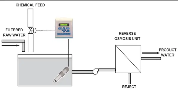
Reverse Osmosis (Fig. 10):
pH control protects Membranes in Reverse Osmosis
Reverse osmosis is a technique for removing dissolved solids from filtered raw water. It is used in a variety of industries to condition water for plant use, or as a first step in the demineralization process.
Fig. 10: Reverse Osmosis
The key factor in reverse osmosis is the condition of the semi-permeable membrane.
A typical membrane material is cellulose acetate, which tends to be degraded by alkaline (high pH) water, resulting in a loss of efficiency.
Precipitation can occur on the process side of the membrane when the raw water contains calcium harness and its pH is in the alkaline range.
To protect the membrane and avoid scaling, the pH of alkaline raw water can be adjusted to the acid side (pH 5.5 is the usual target).
The control action is not difficult since raw water does not typically tend to have major pH fluctuations or load changes (changes in the titration curve).
To accommodate changes in flow rate, flow measurement can be used to trim the pH control.
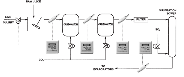
pH Control -Sugar Plants (Fig. 11):
Processed sugar is refined from raw sugar cane.
The process includes the following steps:
wash, crush (or shred), extract (i.e. dissolve in warm water), treat with lime, carbonate, filter, add sulfur dioxide, concentrate, crystallize, and dry. The steps in bold are most critical to the final product and require continuous pH control.
Fig. 11: pH Control in Sugar Plants
Liming:
Alkaline (whitish lime particles suspended in water) is automatically injected to raise the pH of the raw juice to 11-11.5.
The purpose of adding lime (Calcium Oxide) is threefold:-
Neutralize acids in the cane, thereby preventing the sucrose from turning into starch (hydrolysis) or other forms of sugar (inversion).
Precipitate the organic acids into salts for subsequent removal.
Keep foreign matter (insoluble organics, proteins, etc.) in suspension until a filtration process can remove them.
Carbonation:
All traces of lime must be removed before the concentration step to prevent scale buildup.
Carbon dioxide, therefore, is added to the juice to precipitate the lime as less soluble calcium carbonate (limestone), which also tends to capture other impurities during precipitation.
Carbon dioxide is usually added in several stages to avoid an unmanageable type of precipitate that can develop in single-stage carbonation.
At each stage, the pH is measured and carbon dioxide is automatically injected.
By the last stage, the pH should be reduced to about 9.
After carbonation, the juice is filtered to remove all traces of solid particles before flowing to the sulfidation tower.
Addition of Sulfur Dioxide (Sulfidation):
Sulfur dioxide is automatically added to the juice to lower the pH to roughly 5-6 before it goes on to the evaporators.
The sulfur dioxide also bleaches the juice to improve flavor and texture.
Without this step, an alkaline juice would be produced, the sugar crystals would stick together due to excess moisture, and the product would have an undesirable taste.
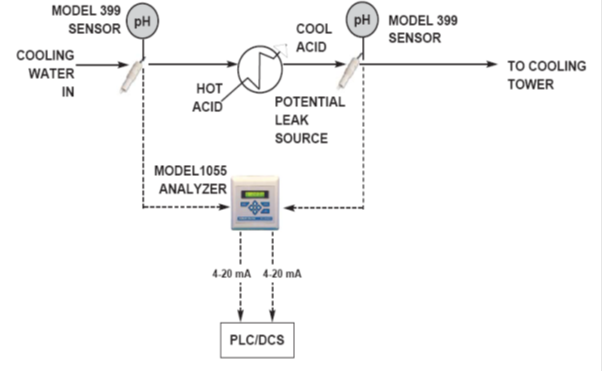
Leak Detection -Using pH measurement (Fig. 12):
Fig. 12: Leak Detection Using pH Measurement
All industries from food and beverage to chemical processing use heat exchangers, condensers, or jacketed vessels.
Leakage of the process into the cooling water represents a loss of product and can be a source of fouling or corrosion in the cooling water system.
Conversely, leakage of the cooling water into the process can be a source of contamination, which is not acceptable.
Differential pH involves using two pH analyzers, one before the potential leak source and one after. The difference in pH is measured and used to detect the leak.
The reason for using differential pH is to cancel out variations in the sample pH.
Ideally, when no leak is occurring the differential pH would read zero.
In a real sense, two factors must be taken into account before applying differential pH. The first is the rate at which the sample pH changes and the second is the transit time, which is the time it takes the sample to pass through the potential leak source
In piping instrumentation, LC and LG refer to two different types of level measurement devices:
LC: LC stands for “level controller” or “level control switch”. This is a device that is used to monitor the level of a liquid in a tank or vessel and control the filling or draining of the tank based on the desired level. The LC typically sends a signal to a control system or actuator to open or close a valve based on the level of the liquid.
LG: LG stands for “level gauge” or “level indicator”. This is a device that is used to visually or electronically display the level of a liquid in a tank or vessel. The LG typically consists of a glass or plastic tube that is mounted on the side of the tank and filled with liquid. As the level of the liquid changes, the level in the tube changes, allowing the operator to easily monitor the level of the liquid.
Both LC and LG devices are commonly used in industrial and process piping systems to monitor and control the level of liquids in tanks and vessels. By providing accurate and reliable level measurement, these devices help to ensure the safe and efficient operation of the system.
This article shall be applied to process engineers’ preparation of basic requirements to enable the piping engineers to finalize LC-LG Arrangements. LC-LG arrangements should be prepared through engineers in process engineering, control engineering, piping engineering, and the mechanical engineering department’s close collaboration. Total coordination should be executed by the piping engineer.
Work Step of LC-LG Arrangement
The piping Engineer should prepare a datasheet based on the skeleton drawings. The following items shall be filled.:
① Vessel Item Number
② Service
③ Instrument Tag Number
④ P&ID Numbers
⑤ Dimensions of Equipment
(Prepare a sketch of the Equipment outline and liquid levels) Then, the datasheet shall be sent to the process department.
Process condition shall be filled in, and visible range/control range shall be indicated by Process Engineer
① Design Pressure & Temperature
② Operating Pressure & Temperature
③ Fluid Name
④ Operating Specific Gravity
⑤ Visible range
⑥ Control range, if required
Then, the data
sheet shall be sent to the control engineering department.
The instrumentation Engineer will select the LC type according to the detailed engineering design data of instrumentation, and the following data shall be filled in.
① Quantity of level instrument
② Type of level instrument
③ Length (Center to center, Visible range)
④ Connection Size / Rating
⑤ Line Class
Then, the datasheet shall be sent to the piping department.
Now piping engineers will select LG type based on process condition, and the following data shall be filled in.
① Quantity of Level Gauge
② Type of Level Gauge
Decide the nozzle height and valve assembly. Such information shall be indicated on the datasheet.
Then, the data
sheet shall be distributed to the disciplines concerned.
The mechanical Engineer will check interference between the nozzle welding line and the equipment welding line. If any, nozzle height shall be adjusted by the piping engineer.
Finally, the LC-LG arrangement shall be followed to P&ID by Control/Instrumentation Department
LC-LG Design Criteria
Fluid conditions:
The fluid name shall be specified.
Polymerization, fouling, slurry, and other data required for the selection of LCs and LGs which are not indicated on P&IDs shall be entered in the process data sheets.
In the case of multi-phase fluid, the specific gravity of the individual fluid shall be entered.
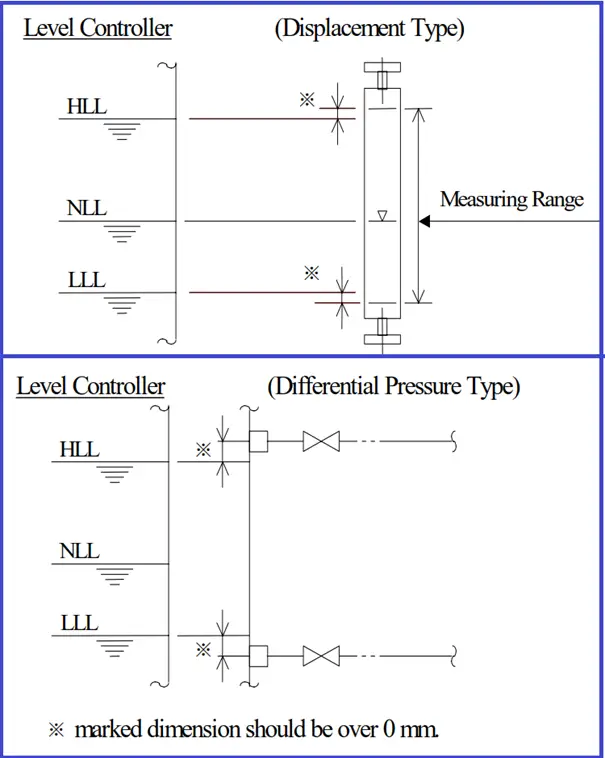
Level Control (LC)
The typical arrangements of level instruments are indicated below in Figure 1.
Fig. 1: Typical Arrangements of Level Instruments
The external covered displacement type or deferential pressure type level instrument should be selected on the following basis:
Visible length over 1200 mm(4FT) : Deferential Pressure Type
Differential pressure of differential pressure type level instrument should be recommended over 500 mm H2O. (Measuring range ≧ 500/Sp Gr)
The diaphragm seal type is recommended for corrosive fluid.
The external displacement type shall not be used for flashing services or averted external radiation services.
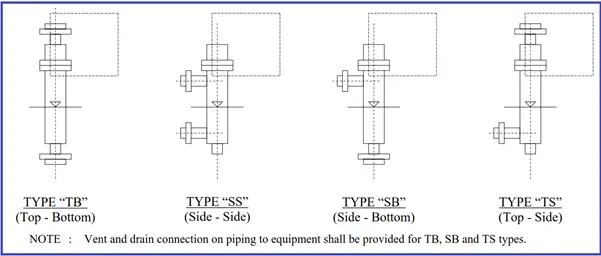
If displacement types are to be used, their installation types shall be entered according to the fluid properties and the client’s instructions, etc. Normally, side-side(“SS”) LCs shall be used.
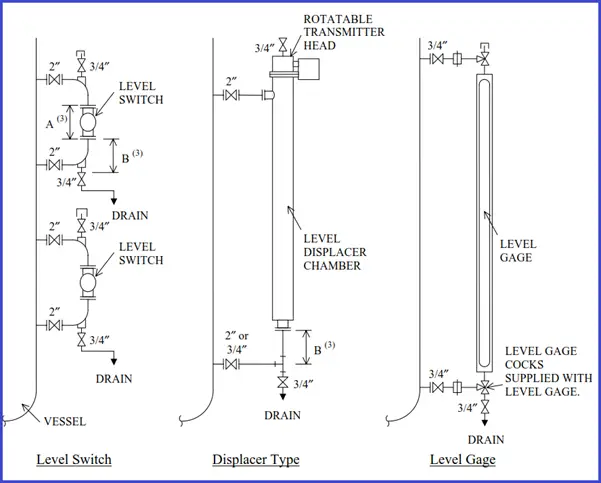
Connection Type of Displacement Level Instruments
Fig. 2: Level Instruments
Level Switch (LS)
LS and LC should be installed on the same standpipe. However, LS and LC shall be installed separately for cloggy services.
The type of LS should basically be external ball float or displacement type.
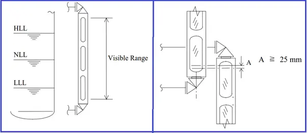
The visible range of LG shall cover the control range of LC.
In the following services, through vision type gage glass should be used.
Liquid-liquid interface
Fluid under 20° API
Crude or residue oil
Fluid includes gum or sediments
If the measuring range is large for covering with one LG, two or more LG shall be used. However, the visible range of each LG shall be overlaid as follows:
Fig. 3: Level Gage
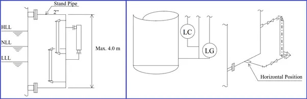
If the plural numbers of LGs are needed, the standpipe can be used. The standard size of the standpipe connection should be 2 inches and the maximum length of the standpipe shall be 4 m. If the standpipe length is over 4 m, the standpipe size should be increased.
In the case of standpipe connection and Low Liquid Level (LLL) is very close to the vessel welding line,LG can be connected at the same level of the horizontal portion of standpipe.
Fig. 4: LC LG Arrangement
Connections to vessel -Level instrument connections shall be made directly to vessels and not to process flow lines or nozzles (continuous or intermittent) unless the fluid velocity in the line is less than 0.6 m/sec (API Recommended Practice 551). Connections and interconnecting piping should be installed so that no pockets or traps can occur.
Level Instruments Mounted Direct to Vessel
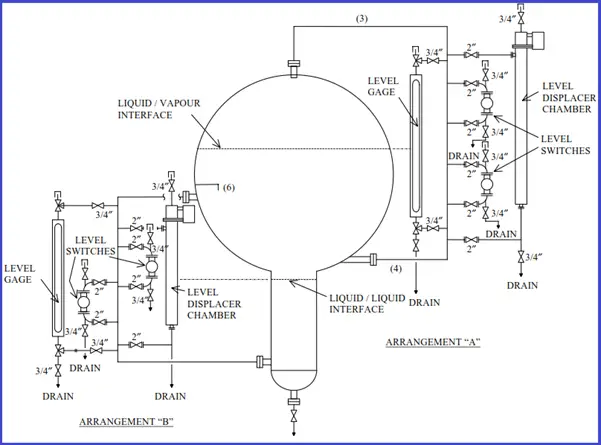
The typical arrangements of the level instruments to be mounted directly to the vessel are as follows:
Fig. 5: Level Instruments in Vessel
Level Instruments on Standpipe: Typical Arrangement-
Fig. 6: Level Instruments on Stand Pipe
Recommended LC LG Arrangement
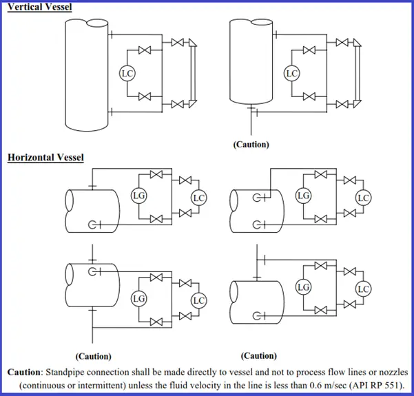
The typical LC and LG arrangements are shown in the figures below:
Fig. 7: Recommended LC LG arrangement for vertical and horizontal Vessels
Seismic Analysis of Piping Systems: Earthquake Analysis
Seismic Analysis of piping systems is performed to safeguard the piping systems from unforeseen earthquake events. During the initial design phase, based on earlier earthquake data available in codes and standards, piping systems and civil structures are designed to withstand piping movements during seismic events. The ASME B31 codes provide the allowable stresses for seismic analysis of piping systems. An equivalent static seismic analysis is the most preferred method, even though dynamic analysis is possible.
Piping Seismic Analysis Basis
The criteria for line selection for seismic analysis are normally mentioned in the ITB documents if the construction site falls under the seismic zone. If the same is not mentioned then the following lines can be considered:
Lines with an outside diameter of 6” and larger.
Transfer lines/Two-phase flow lines.
Piping systems connected to Strain-sensitive equipment like Compressor, Turbine, and Pump.
Other lines are considered important as per the stress engineer’s decision.
Advantages of Seismic Analysis of Piping Systems
During a seismic or earthquake event, the piping system and components can lead to catastrophic failure if proper seismic analysis of piping systems is not performed during the design stage. So, earthquake analysis of piping systems must be performed while piping stress analysis if the plant falls under seismic zones as specified by codes. The advantages that a proper seismic analysis of the piping system offers are
The system will be properly supported for earthquake events. So major system failure is prevented.
The seismic analysis assists in identifying the limits and restrictions of the available design codes and standards.
Civil structures will be designed accounting for piping seismic loads so robust design.
Seismic design help piping engineers improve their ability to model the piping system behavior for a particular ground motion.
Stress Allowable Values for Piping Seismic Analysis
As per code ASME B31.3, the longitudinal stresses generated due to sustained and occasional loads should be within 1.33 times Sh (Basic allowable stress at hot temperature) value. So We have to add Sustained stress and occasional stress such that the scalar combination of the same remains within the limit specified by the code. Normally nozzle load checking is not required for seismic analysis. However few companies need the nozzle load checking at the seismic condition for static equipment. Sometimes the allowable nozzle load can be increased by 50% for checking in occasional cases. However, nozzle load checking is not required in the seismic case for rotating equipment. The following article will describe steps to perform the static method of seismic analysis in Caesar II.
Seismic Analysis of Piping System using Caesar II
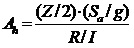
The first step in the static seismic analysis is to collect the seismic coefficient. Sometimes the value of the seismic coefficient is provided directly and sometimes enough data is provided to calculate the same. The following equation (as per IS 1893) can be used to calculate the seismic co-efficient:
Here
Spectral Acceleration Coefficient (Sa/g) = 2.5 (Examples are shown for the sake of a typical value calculation)
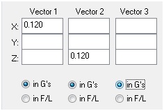
This co-efficient value needs to be entered in the Caesar spreadsheet as shown below:
Caesar Spreadsheet showing the input of Seismic Co-efficient
Normally the Y component is not entered. However, few clients may require the input of the same. in that case, follow the guidelines provided by them.
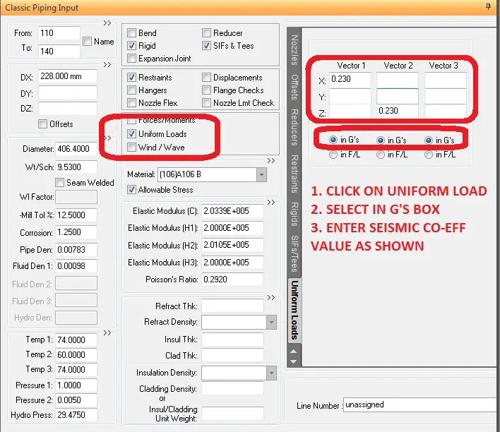
To perform seismic analysis open the Caesar II spreadsheet and click on uniform loads as shown in the below-mentioned figure.
Caesar II Spreadsheet showing Seismic Analysis
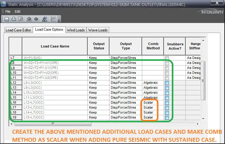
Load Cases for Static Seismic Analysis
After that prepare the load cases for seismic analysis. The load cases normally prepared are shown in the figure attached below:
Load Cases for Seismic Analysis
Checking Output of Seismic Analysis
Once you prepared the required load cases simply run the file and check the stresses for Code compliance as mentioned below:
Caesar Output window for Seismic Analysis
Check the restraint summary for load cases L8 to L11 in the above-mentioned figure and check stresses for load cases L16 to L19.
The above method explained is the equivalent static method of seismic analysis for piping systems. The earthquake analysis can also be performed using the dynamic spectrum method in which a dynamic spectrum must be generated for analysis.