ANSI Pump and API Pump are two types of Centrifugal pump styles that are used in Chemical Plants, Refineries, and Oil and Gas Industries. They have some distinct differences. This article will compare the major features of both these pumps.
What is an API Pump?
An API Pump is a special type of centrifugal pump that meets the design, inspection, and testing criteria specified by the American Petroleum Institute’s API-610 standard for pumps. In Refineries and Petrochemical Industries, mostly API pumps are used as they provide very good operating experience in handling hydrocarbons (oil, gasoline, Natural gas, and petroleum products) due to their robust design. Generally, They come in many different forms employing a number of pumping mechanisms. Traditionally API pumps are considered very conservative (stringent) and costly.
What is an ANSI Pump?
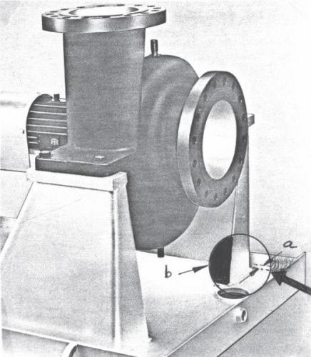
ANSI Pumps are a type of horizontal, single-stage, end suction centrifugal pump that has an overhung impeller and back pull-out. This type of pump is designed based on the ASME B73.1 standard. Due to their low cost, they are popularly used in chemical industries, refineries, and industrial and mining applications for comparatively less temperature pressure applications. The main advantage of ANSI pumps is their interchangeability across manufacturers and brands.
ANSI Pump vs API Pump
Compared to an API pump, the typical ANSI pump has the following characteristics:
Criteria
API Pump
ANSI Pump
Design Code
API 610
ASME/ANSI B 73.1
Pump Casing
Thick Casing, more corrosion allowance. In general, designed for 750 PSIG at 500℉.
Thinner Casing, less corrosion allowance. Normally designed for 300 PSIG at 300℉.
Nozzle Load
More sensitive to pipe-induced stresses, ANSI pumps allow reduced permissible nozzle load
More sensitive to pipe-induced stresses, hence ANSI pumps allow reduced permissible nozzle load
Stuffing Box Size
API pumps have a large Stuffing Box.
Smaller stuffing box size. Unless a large bore option is chosen, an ANSI pump may not be able to accommodate the optimum mechanical seal for a given service.
Impeller Design
API pumps feature closed impellers with replaceable wear rings.
ANSI pump impellers are designed and manufactured without wear rings. Many ANSI pump impellers are open or semi-open
Mounting Option
Normally, API pumps are center-line mounted
Generally, ANSI pumps are foot-mounted.
Application
API pumps are suitable for heavy-duty, much higher temperatures, and pressures
ANSI pumps are usually not suitable for moving thicker and/or viscous fluids. Moderate duty application.
Reliability
API pumps are highly reliable
The reliability of ANSI pumps is comparatively less.
Cost
High
Comparatively less
Difference Between API Pump and ANSI Pump
Refer to the attached sketch. In foot-mounted pumps, casing heat tends to be conducted into the mounting surfaces and thermal growth will be noticeable. It is generally easier to maintain the alignment of API pumps since their supports are surrounded by the typically moderate-temperature ambient environment.
Choosing Pump Type: API or ANSI
The decision on API vs. ANSI construction is experience-based and is not governed by governmental or regulatory agencies. However, experienced machinery specialists have their own likes and dislikes based on the experience gathered by them over their long years in the machinery field.
Many highly experienced and reliability-focused machinery engineers would prefer to use pumps designed and constructed according to API 610 for toxic, flammable, or explosion-proof services at on-site locations in close proximity to furnaces and boilers in some of the conditions (rules-of-thumb) that are listed below:
Head exceeds 106.6 m (350 ft)
The temperature of pumpage exceeds 149°C (300°F) on pumps with discharge flange sizes larger than 4 inches or 177°C (350°F) on pumps with a 4-inch discharge flange size or less.
Driver horsepower exceeds 74 kW (100 hp)
Suction pressure in excess of 516 kPag (75 psig)
Rated flow exceeds flow at best efficiency point (BEP)
Pump speed in excess of 3600 rpm.
The author mentions that there have been exceptions made where deviations from the rules-of-thumb were minor, or in situations where the pump manufacturer was able to demonstrate considerable experience with ANSI pumps under the same, or even more adverse conditions.
Finally, the author gives his opinion on choosing either API or ANSI pumps based on the following:
Conventional Wisdom: API-compliant pumps are always a better choice than ANSI or ISO pumps
Fact: Unless flammable, toxic or explosion-prone liquids are involved, many carefully selected, properly installed, operated and maintained ANSI or ISO pumps may represent an uncompromising and satisfactory choice.
The above comparison that is provided in the article is referenced from Heinz P. Bloch’s book “Pump User’s Handbook Life Extension” co-authored with Allan R. Budris.
Proper pipe selection for a plant is really a difficult task. Organized efforts of Metallurgist and Process Engineers are required for proper pipe selection. There are two approaches to pipe selection that are normally followed in industries.
Selection of Pipe by Pipeline Approach
When pipelines and production facilities are being built the emphasis is placed on the pipe wall thickness. Generally, there is a great amount of pipe, and quantities of fittings and valves are small by comparison. Minimizing the pipe wall is the major economic factor. The extra cost of custom-made fittings is far outweighed by the savings on the pipe. The pipe is purchased by weight, so the added cost of high-strength material to lower the pipe wall is a reasonable consideration. When high-strength material is specified, extra inspection and more stringent interpretation are also necessary. The cost of the extra inspection is also a reasonable consideration. Spare parts warehousing is a small consideration.
Plant Pipe Selection Approach
When plants are built, the pipe selection emphasis is on standardized materials. The design is such that materials made to the specified standard are adequate for the service. Certain specific services may require additional inspection or special requirements, but these are for service, and not economics.
Materials are usually purchased from warehousing companies. The relative cost of pipe is a considerably smaller percentage of the total cost, compared with pipelines. The cost of machinery and equipment takes a large part of the budget. The cost of fittings and particularly valves make up a large part of the whole piping budget. The easy, and quick procurement of spare, and replacement parts, becomes very important. Pipe walls may be bumped up, if the quantity is small, to a greater thickness that is more available or already specified in large quantities. There is a price vs. availability relationship that is easy to overlook.
Pipe Selection Guide: Price vs. Availability
The price vs. availability relation can be shown by the following examples. Type 304 stainless steel costs less than type 316. Many valve manufacturers standardize on type 316 because it is generally suitable for type 304, and 316 services. If type 304 is the only choice, a valve will have a higher price and extended delivery. Even if the price is the same, the lack of availability can slow a project.
The actual material is normally specified by the process licensor, company, or project metallurgist, or is part of the Process Package. The selection of pipe is limited by the design condition and specific service as mentioned below:
Design Limitations while piping selection
Pipe Material:
Pipe material is defined by material, type of joint, joint efficiency, wall thickness, etc. The pipe has a material name. Typical names are carbon steel, stainless steel, and chrome-moly steel. The pipe has a material type. Typical types within the material names are killed steel, low-temperature carbon steel, carbon steel, austenitic stainless steel, ferritic stainless steel, type 316 stainless steel, 11/4 Cr – 1/2 Mo, and so on.
The pipe has a manufacturing standard. Typical material standards for pipe are ASTM A106, API 5L, ASTM A333, and ASTM A671, for carbon steel, ASTM A312, and ASTM A358, for stainless steel, and ASTM A355, and ASTM A691. Again each Pipe has a material grade. Typical grades are Grade B, X60, TP304, and Gr 11/4 Cr.
Pipe Sizes:
The outside diameter of the steel pipe shall be in accordance with API Spec 5L Table 6.2. Intermediate sizes and the sizes NPS 1/8, 1/4, 3/8, 1-1/4, 2-1/2, 3-1/2, and 5 shall not be used except when necessary to match equipment connections. In this case, a suitable transition shall be made as close as practical to the equipment.
The minimum allowable pipe size, including vents and drains, is NPS 3/4.
Wall Thickness of Pipe:
The standard for Wall Thickness: Wall thickness may be expressed as wt, std, xs, and XXS, schedule, and plate thickness. Weight classes and schedules are defined in ASTM A53.
Pipe Made From Plate: A pipe made from a plate shall have the wall thickness expressed in mm.
Minimum Wall Thickness: The minimum wall thickness for the pipe is generally the minimum thickness that will stand under its own weight, with minimum deflection. Wall thickness is always calculated for the design temperature and pressure, in accordance with the appropriate ASME B31 code.
Wall Thickness Standardization: Wall thickness standardization is necessary to minimize stocking requirements, and take advantage of quantity pricing. In the plant approach, the pipe is not specified in a vacuum. The pipe is welded to flanges and fittings in relatively large quantities. The major criterion in pipe wall selection may not be from temperature and pressure, but from the availability of fittings and flanges. Piping is a system, and other items must be considered during selection. When a pipe is made from a plate, the accompanying fittings may be in a special order, and affect the critical path.
Piping End Connections:
Threaded End Pipe:Threaded pipe shall be provided threaded and coupled.
Pipe for Socket weld Systems: Pipe intended for socket welding shall be square cut.
Butt-welding Ends: Butt welding ends shall be in accordance with the requirements of ASME B16.25.
Lengths: Pipe shall be supplied in double random lengths.
Galvanizing: Galvanizing shall be applied in accordance with ASTM A53.
Pipe Joints:
Seamless Pipes:
Wrought Pipe:Seamless pipe is made by extrusion, or by piercing and rolling
Casting: Cast pipe suitable to be qualified as seamless must be centrifugally cast.
Forging: Seamless pipe can be made by the forging and boring process.
ERW Pipe:
ERW pipe is Electric Resistance Welded. In this process, a flat plate is formed into a cylinder and put through energized rollers that press the seam together and provide a resistance weld. ERW pipe has reduced allowable than seamless.
EFW Pipe:
Electric Fusion Welded Pipe: EFW pipe is rolled into a cylinder and welded with filler material. This is a fusion weld and may be qualified to several levels.
DSAW: Submerged Arc Welding is a common form of EFW. Depending on thickness, the manufacturing standard calls for a single or double weld. The thinner walls are welded outside, and thicker walls are welded inside and outside, hence Double Submerged Welding, or DSAW.
Type-F: Furnace butt-welded pipe, also known as type F, is used in petrochemical applications only for water.
Straight Seam:
Straight seam refers to a straight seam parallel to the longitudinal axis. The hoop stress has no component in the axial direction. A straight seam is made by drawing a plate through a series of rollers to make it a cylinder, for welding.
Spiral Seam:
A spiral welded pipe is made in a special machine that takes coiled steel and rolls it into a spiral, which is welded into a pipe. This is a relatively continuous process. The machine makes it relatively easy to change pipe size. The convertibility of the machine and the limited stock required make this machine ideal for local production. Spiral welded pipe is not readily accepted in the industry for other than water, despite the favorable cost, and recent tightening-up of the standard.
Joint Efficiency of Pipe:
All pipes that are not seamless are subject to joint efficiency. The committees that publish the codes place a restriction on the allowable stress for the welded pipe. This restriction is in the form of a joint efficiency, clearly stated in the codes.
A pipe can be qualified for higher joint efficiency by inspection. The major factor is radiography. The type and extent of radiography are listed in the codes.
Special Requirements during pipe selection
There may be special requirements for the base material, fabrication, or inspection. These special requirements shall be clearly indicated in the Purchase Description.
Mill Test and Chemical Analysis Report:
A certified mill test and chemical analysis report shall be submitted by the Seller of all alloy pipe (including ASTM A333), and all pressure-containing alloy piping components made from pipe not clearly marked in accordance with MSS SP-25.
A certified mill test and chemical analysis report are also required for carbon steel pipe, nipples made from pipe, swages, and all pressure-containing carbon steel components made from pipe not clearly marked in accordance with MSS SP-25, for use in ASME Section I or ASME B31.1 piping systems.
When alloy material and carbon steel, as noted above, are purchased by an outside shop pipe spool fabricator, the fabricator shall obtain these reports.
Piping Nipples:
Pipe Nipples with schedule 160 shall be installed in sizes NPS 2, and smaller pipe sizes in vibration service where bracing cannot be effectively provided.
Piping Material Classes:
The piping material classes in these standards show the actual selections for piping, as well as all piping materials, by example. The classes show pipe and all of the associated materials for each service. These classes are to be used as a basis for new services.
Pipe Selection with Specific Service Limitations
Carbon Steel Pipes:
Carbon steels are used in a variety of cases.
Low-Strength Steel: Low-strength steels are generally only used for open piping, such as gravity sewers.
Regular Steel: Regular steels are used for general service, including water, and hydrocarbons. These are services with no special requirements.
Low-Temperature Carbon Steel:Low-temperature carbon steel is steel that has been killed to improve the microstructure to raise the fracture toughness, to reduce susceptibility to brittle fracture. Low-temperature carbon steel must be qualified by impact testing.
Killed Steel: Killed steel has the same improved microstructure as low-temperature carbon steel, but the improved microstructure reduces susceptibility to sulfide cracking, as well as other related cracking. The fine grain structure and quality of structure also provide resistance to hydrogen attack.
NACE: When a pipe is to be used in wet H2S, NACE MR0175 is invoked to assure resistance to sulfide cracking, including the use of killed steel.
High-Strength Steel: High-strength steels are generally not approved for use under ASME B31.1 and B31.3. only the lowest grades are listed. High-strength steels are used in pipeline service to reduce the pipe wall.
Chrome alloys:
Corrosion Resistance: Chromium alloy steel also uses molybdenum to control the microstructure. Corrosion resistance is improved.
Hydrogen Resistance: Generally, chrome and Molybdenum are added for hydrogen resistance. The Nelson Curves show the relationship between the partial pressure of hydrogen, temperature, and chrome content. The curves are found in API 941.
High Strength: The addition of chrome also improves high-temperature strength.
High Temperature: Steam will cause graphitization in carbon steel at temperatures over 425 deg. C and chrome steel is recommended.
Stainless Steel Pipes:
Stainless Steel Types: Stainless steel offers resistance to corrosion in three ways. Higher percentages of Chromium offer corrosion resistance, as an alloy. Higher percentages of chrome with nickel alter the microstructure from ferrite to austenite. The austenite offers corrosion protection. Certain compositions will produce what is known as duplex steel, which exhibits the qualities of ferritic and austenitic steels.
300 Series Steels: The 300 series steels are the most common. There are two basic subtypes, in which the austenite is stabilized, or not. The most common types are type 304 and type 316. These materials exhibit microstructure problems at various temperatures. The austenite can be stabilized with Titanium, and Columbium (Niobium). These grades are type 321 and 347. A metallurgist is required to make the determination. 300 series stainless steels are extremely susceptible to chloride stress cracking.
400 Series Steels: The 400 series steels are less available, and are more difficult to work with. These steels are generally only specified for specific fluid conditions. 400 series steels offer less corrosion resistance than 300 series. Ferritic stainless steel offers better abrasion resistance than the 300 series.
Duplex Steels:Duplex stainless steels have the corrosion resistance of the 300 series, and the abrasion resistance of the 400 series, and are not subject to chloride cracking.
Other Materials:
Some of the materials below are represented by the proprietary name for clarity.
Monel:Monel is a copper-nickel alloy that is usually used around caustic, at higher temperatures. Monel is not readily available, particularly valves.
Alloy 20: Alloy 20 is a proprietary name, but most alloys have similar names. Alloy 20 is most used in acid services.
Nickel Alloys: Nickel alloys such as Incoloy and Inconel are proprietary, and are used for high-temperature services.
Pipe for Pipelines:
With the pipeline approach, the material is usually high strength. The specific composition of the metal depends on the makeup of the fluid carried. The limitations on composition vary, so there is a separate specification specifically for line pipe. Schedule 40 is usually considered the minimum pipe wall, for mechanical strength, in small sizes, NPS 10 and smaller. When the pipe wall calculates at or below Sch 40, regular strength material is a considerable cost saving.
Spring hangers: Common Interview Questions with Answers
Most of the highly critical stress systems employ one or more Spring Hangers in Stress systems. This article explains the frequently asked spring hanger questions with answers:
What is the main difference between Constant and Variable Spring Hanger? When to use these hangers?
Ans: In Constant Spring hanger the load remains constant throughout its travel range. But In variable Spring hangers, the load varies with displacement. Spring hangers are used when thermal displacements are upwards and the piping system is lifted off from the support position.
A variable spring hanger is preferable as this is less costly. Constant springs are used:
a) When thermal displacement exceeds 50 mm
b) When variability exceeds 25%
c) Sometimes when piping is connected to strain-sensitive equipment like steam turbines, centrifugal compressors, etc and it becomes very difficult to qualify nozzle loads by variable spring hangers, constant spring hangers can be used.
What do you mean by variability? What is the industry-approved limit for variability?
Ans: Variability= (Hot Load-Cold load)/Hot load= Spring Constant*displacement/Hot load. The limit for variability for variable spring hangers is 25%.
What are the major parameters you must address while making a Spring Datasheet?
Ans: Major parameters are: Spring TAG, Cold load/Installed load, Vertical and horizontal movement, Piping design temperature, Piping Material, Insulation thickness, Hydrotest load, Line number, etc.
How to calculate the height of a Variable Spring hanger?
Ans: Select the height from the vendor catalog based on spring size and stiffness class. For the base-mounted variable spring hanger, the height is mentioned directly. It is the spring height. For top-mounted variable spring hangers ass spring height with turnbuckle length, clamp/lug length, and rod length.
Can you select a proper Spring hanger if you do not make it program defined in your software? What is the procedure?
Ans: In your system first decide the location where you want to install the spring. Then remove all nearby supports which are not taking the load in the thermal operating case. Now run the program and the sustained load on that support node is your hot load. The thermal movement in that location is your thermal movement for your spring. Now assume a variability for your spring. So calculate Spring constant=Hot load*variability/displacement. Now with spring constant and hot load enter any vendor catalog to select a spring inside the travel range.
Why horizontal displacement is specified in the datasheet? What will you do if the angle due to displacement is more than 4 degrees?
Ans: For bottom-mounted springs it is mentioned to avoid large spring bending by frictional force and displacement. So that additional measures can be taken to lower frictional force by providing PTFE/graphite slide plate. For top-mounted spring hangers horizontal displacement is mentioned to check angularity of 4 degrees to reduce transmission of horizontal force to piping systems as spring hangers are designed to take the vertical load only. If the angle becomes more than 4 degrees due to large horizontal movement then install the spring hanger in an offset position so that after moving the angle becomes less than 4 degrees.
Which spring will you select for your system: Spring with low stiffness or higher stiffness and why?
Ans: Springs with lower stiffness provide less load variation for the same travel. So this spring is a better choice than a spring hanger with higher stiffness.
Excavation is a fundamental part of many construction projects, from building foundations to laying infrastructure. However, while excavation is essential, it also comes with significant hazards that can lead to serious accidents if not properly managed. Excavation Hazards are the dangers associated with soil excavation at construction sites. During construction site excavation, both the workers inside trenches and on the surface are at high risk. So protective measures must be considered against the hazards in the excavation. In this article, we will explore different types of excavation hazards during site excavation and the protective measures that should be undertaken to reduce accidents.
Definitions related to Excavation Hazard
Excavation – a man-made cut, cavity, trench, or depression formed by earth removal.
Trench – a narrow excavation. The depth is greater than the width but not wider than 4.5 meters.
Shield – a structure able to withstand a cave-in and protect employees
Shoring – a structure that supports the sides of an excavation and protects against cave-ins
Sloping – a technique that employs a specific angle of incline on the sides of the excavation. The angle varies based on an assessment of impacting site factors.
The discussion of this topic covers four main points. At the conclusion of this article, you should be able to:
State the greatest risk present at an excavation.
Briefly describe the three main methods for protecting employees from cave-ins.
Name at least three factors that pose a hazard to employees working in excavations and at least one way to eliminate or reduce each of the hazards.
Describe the role of a competent person at an excavation site.
Types of Excavation Hazards
Excavation is the removal of soil or rock from a construction site that creates an open space for installing pipes, equipment, etc. using various construction tools, machinery, or explosives. So, excavation creates a hole or cavity that is hazardous. Various types of excavation hazards arise at the construction site. Cave-ins or collapses are the greatest risks. Other hazards include:
Asphyxiation due to lack of oxygen
Inhalation of toxic materials
Fire
Excavated Soil or Equipment falling on workers.
Moving machinery near the edge of the excavation can cause a collapse.
Falling, Slips, Trips
The accidental severing of underground utility lines/power lines.
Material handling Hazards.
Excavation is one of the most hazardous construction activities. Most accidents occur in trenches 1.2 to 4.5 meters deep. There is usually no warning before a cave-in.
1. Cave-ins
Cave-ins are perhaps the most dangerous excavation hazard. They occur when the walls of a trench or excavation site collapse, burying workers under tons of soil.
1.1 Reasons of Cave-ins
The main causes of cave-ins include:
Unstable Soil: Soil types such as sandy or loose soils are more prone to collapse. Clay and silt can also become unstable when wet.
Improper Shoring: Shoring systems (support structures) that are incorrectly installed or inadequate can fail, leading to cave-ins.
Water Accumulation: Rain or groundwater infiltration can weaken soil stability, increasing the risk of cave-ins.
Vibration: Nearby construction activities or heavy traffic can cause soil to shift and destabilize excavation walls.
1.2 Precautions from Excavation Hazards, Cave-ins
Employees should be protected from cave-ins by using an adequately designed protective system. Protective systems must be able to resist all expected loads to the system.
1.3 Protective system from Cave-ins
A method of protecting employees from cave-ins, from material that could fall or roll from an excavation face or into an excavation, or from the collapse of adjacent structures. Protective systems include
support systems,
sloping and benching systems,
shield systems, and
other systems that provide the necessary protection.
Additionally, the following measures should be undertaken:
Soil Analysis: Conduct a thorough soil analysis to determine soil type and stability.
Shoring and Shielding: Use proper shoring (bracing) and shielding systems designed for the specific excavation depth and soil conditions.
Drainage Systems: Implement effective drainage solutions to manage water accumulation.
Regular Inspections: Conduct regular inspections of excavation sites to identify and address potential hazards.
1.4 Excavation Safety Plan Requirements
A well-designed protective system means
Correct design of sloping and benching systems.
Correct design of support systems, shield systems, and other protective systems.
Appropriate handling of materials and equipment.
Attention to correct installation and removal.
Several factors come into play when developing a total protective system. The design of the system itself, how materials and equipment are handled in and around the excavation, and the installation and removal of protective system components.
1.5 Design of Protective Systems against Excavation Hazards and Risks
The employer shall select and construct :
slopes and configurations of sloping and benching systems
support systems, shield systems, and other protective systems
Shield – can be permanent or portable. Also known as trench box or trench
Shoring – such as a metal hydraulic, mechanical, or timber shoring system that supports the sides
Sloping – from sides of an excavation that are inclined away from the excavation
1.6 Protect Employees Exposed to Potential Cave-ins
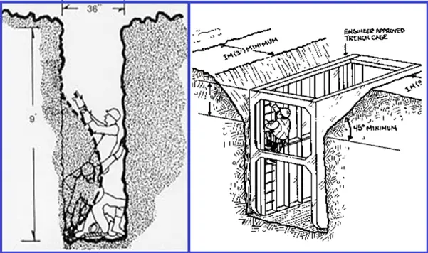
To protect personnel from cave-in excavation hazards (Fig. 1) the following preventive measures can be undertaken
Maintain at least a 2 m distance from the edge of the cut and use blocks to prevent over-run.
Slope or bench the sides of the excavation,
Make proper arrangements to barricade the area being excavated.
Support the sides of the excavation, or
Place a shield between the side of the excavation and the work area
Fig. 1: Excavation and Hazards
1.7 Controlling Factors for Excavation Protective System
Various factors need to be considered while designing a protective system against the hazards and risks of excavation. Those are
Soil classification
Depth of cut
The water content of the soil
Changes due to weather and climate
Other operations in the vicinity
The employer or his designee must select and construct designs of support systems, shield systems, and other protective systems.
Trenches more than 5 feet require shoring or must have a stabilized slope
Trenches less than 5 feet – a competent person must inspect to determine that a protection system is not necessary for soils where there is no indication of a potential cave-in
In hazardous soil conditions, trenches under 5 feet need protection
1.8 Shoring in Construction
Shoring in construction means erecting a temporary structure to support unsafe excavation walls or other unsafe structures till work is finished.
Provides a framework to work in
Uses Wales, cross braces, and uprights
Supports excavation walls
Must know the soil type
Must know the depth and width of the excavation
Must be familiar with the OSHA or other relevant standard Tables
Trench Shield: A trench shield must be built around the work area.
1.9 Hydraulic Trench Support
Using hydraulic jacks the operator can easily drop the system into the hole. Once in place, hydraulic pressure is increased to keep the forms in place. Trench pins are to be installed in case of hydraulic failure
1.10 Materials and Equipment
Materials and equipment used for protective systems shall be free from damage or defects that might impair their proper function.
Manufactured materials and equipment used for protective systems shall be used and maintained in a manner that is consistent with the recommendations of the manufacturer, and in a manner that will prevent employee exposure to hazards.
When material or equipment that is used for protective systems is damaged, a competent person shall examine the material or equipment and evaluate its suitability for continued use. If the competent person cannot assure the material or equipment is able to support the intended loads or is otherwise suitable for safe use, then such material or equipment shall be removed from service and shall be evaluated and approved by a registered professional engineer before being returned to service.
1.11 Protection from Vehicles during excavation
Install barricades
Hand/mechanical signals
Stop logs
Grade soil away from the excavation
Fence or barricade trenches left overnight
1.12 Hazardous Conditions
The weight and vibrations of the crane make this a very hazardous condition.
They should not be working under this crane.
In addition to the unprotected trench, a cave-in hazard is increased by machinery which gets too close.
Even normal vehicular traffic, such as that along an adjacent interstate or road through an industrial part may impact an excavation. The vibrations from continuous or heavy traffic may undermine the soil and cause a cave-in.
1.13 Excavation Spoils
Excavation spoils are the soil, dirt, and rubble that are removed while excavating. The following considerations should be made for preventing hazards from excavation spoils.
Don’t place spoils within 2 feet of the edge of an excavation
Measure from the nearest part of the spoil to the excavation edge
Place spoils so rainwater runs away from the excavation
Place spoil well away from the excavation
2. Other Excavation Hazards
2.1 Falling Loads
Falling loads involve materials or equipment falling into an excavation site, which can pose severe risks to workers. Causes include:
Improper Material Storage: Materials stored too close to the edge of an excavation can fall in.
Equipment Movement: Construction equipment near the excavation site can accidentally drop loads.
Unsecured Loads: Loads that are not properly secured can shift and fall.
2.1.1 Preventative Measures from Falling Loads:
Secure Storage: Keep materials and equipment well away from the edge of excavations.
Use Barriers: Install barriers or guardrails to prevent accidental falls of materials.
Proper Training: Ensure that workers handling equipment are trained in secure load practices.
2.2 Falling into Excavations
Workers and pedestrians can accidentally fall into excavations if proper safeguards are not in place. This can result in severe injuries or fatalities.
2.2.1 Preventative Measures from Falling into Excavations:
Guardrails and Covers: Install guardrails and covers around excavation sites to prevent falls.
Warning Signs: Place clear warning signs around excavation areas.
Access Control: Restrict access to excavation sites to authorized personnel only.
2.3 Utility Strikes
Excavation work often intersects with existing utilities such as gas, water, or electrical lines. Striking these utilities can lead to dangerous situations such as explosions, floods, or electrocution.
2.3.1 Preventative Measures from Utility Strikes:
Utility Locating: Use utility locating services to map out existing underground utilities before digging.
Safe Digging Practices: Employ safe digging practices, such as hand digging near known utility lines.
Emergency Procedures: Develop and communicate emergency procedures for utility strikes.
2.4 Equipment Hazards
Excavation work involves various types of equipment, including backhoes, excavators, and bulldozers. Hazards associated with equipment include:
Equipment Overturns: Heavy machinery can overturn if used improperly or if the ground is unstable.
Moving Parts: Equipment with moving parts can cause injuries if proper safety precautions are not followed.
Blind Spots: Equipment operators may have limited visibility, increasing the risk of accidents.
2.4.1 Preventative Measures from Equipment Hazards:
Operator Training: Ensure that all equipment operators are properly trained and certified.
Maintenance: Regularly maintain and inspect equipment to ensure it is in good working condition.
Safety Measures: Use spotters to guide equipment operators and maintain clear communication on-site.
2.5 Exposure to Hazardous Atmospheres
Excavations, especially those of significant depth, can sometimes encounter hazardous atmospheres, including toxic gases, low oxygen levels, or high levels of particulates.
2.5.1 Preventative Measures from Exposure to Hazardous Atmosphere:
Air Monitoring: Use air monitoring equipment to check for hazardous atmospheric conditions.
Ventilation: Implement proper ventilation systems to ensure a safe working environment.
Protective Equipment: Provide workers with appropriate personal protective equipment (PPE) such as respirators.
Test excavations more than 1.2 meters before an employee enter the excavation for:
Oxygen deficiency
High combustible gas concentration
High levels of other hazardous substances
Employees shall not be permitted to work in hazardous and/or toxic atmospheres. Such atmospheres include those with:
less than 19.5% oxygen,
a combustible gas concentration greater than 20% of the lower flammable limit, and,
concentrations of a hazardous substance that exceed those specified in the Threshold Limit Values for airborne contaminants established by the ACGIH.
2.6 Preventing Excavation Hazards from Water
Water is Hazardous. So,
Employees shall not work in excavations in which there is accumulated water, or in excavations in which water is accumulating unless adequate precautions have been taken to protect employees against the hazards posed by water accumulation. The precautions necessary to protect employees adequately vary with each situation but could include special support or shield systems to protect from cave-ins, water removal to control the level of accumulating water, or the use of a safety harness and lifeline.
If water is controlled or prevented from accumulating by the use of water removal equipment, the water removal equipment and operations shall be monitored by a competent person to ensure proper operation.
If excavation work interrupts the natural drainage of surface water (such as streams), diversion ditches, dikes, or other suitable means shall be used to prevent surface water from entering the excavation and to provide adequate drainage of the area adjacent to the excavation.
Water = Cave-in Hazard
2.7 Means of Egress
A stairway, ladder, or ramp must be present in excavations that are 1.2 meters or deeper
Structural ramps that are used solely by employees as a means of access or egress from excavations shall be designed by a competent person. Structural ramps used for access or egress of equipment shall be designed by a competent person qualified in structural design and shall be constructed in accordance with the design.
Ramps and runways constructed of two or more structural members shall have the structural members connected together to prevent displacement.
Structural members used for ramps and runways shall be of uniform thickness.
Cleats or other appropriate means used to connect runway structural members shall be attached to the bottom of the runway or shall be attached in a manner to prevent tripping.
Structural ramps used in lieu of steps shall be provided with cleats or other surface treatments o the top surface to prevent slipping.
2. 8 Protection from Falls, Falling Loads, and Mobile Equipment
Install barricades
Use hand / mechanical signals
Grade soil away from the excavation
Fence or barricade trenches left overnight
Use a flagger when signs, signals, and barricades are not enough protection
To protect employees from these hazards, take the following precautions:
Keep materials or equipment that might fall or roll into an excavation at least 2 feet from the edge of excavations, or have retaining devices, or both.
Provide warning systems such as mobile equipment, barricades, hand or mechanical signals, or stop logs, to alert operators of the edge of an excavation. If possible, keep the grade away from the excavation.
Provide scaling to remove loose rock or soil or install protective barricades and other equivalent protection to protect employees against falling rock, soil, or materials.
Prohibit employees from working on faces of sloped or benched excavations at levels above other employees unless employees at lower levels are adequately protected from the hazard of falling, rolling, or sliding material or equipment.
Prohibit employees under loads that are handled by lifting or digging equipment. To avoid being struck by any spillage or falling materials, require employees to stand away from vehicles being loaded or unloaded. If cab vehicles provide adequate protection from falling loads during loading and unloading operations, the operators may remain in them.
Competent Person against Excavation Hazards
Must have had specific training in and be knowledgeable about:
Soils classification
The use of protective systems
The requirements of the standard
Must be capable of identifying hazards, and authorized to immediately eliminate hazards
Inspections of Excavations
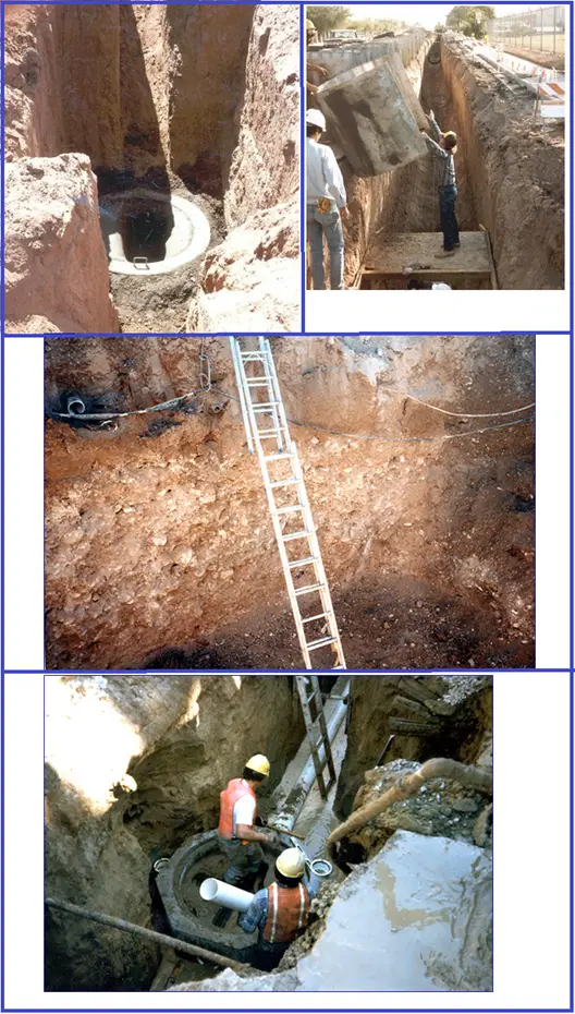
A competent person must make daily inspections (Fig. 2) of excavations, areas around them, and protective systems:
Before work starts and as needed,
After rainstorms, high winds, or other occurrences which may increase hazards, and
When you can reasonably anticipate an employee will be exposed to hazards.
Fig. 2: Inspection
If the competent person finds evidence of a possible cave-in, indications of failure of protective systems, hazardous atmospheres, or other hazardous conditions:
Exposed employees must be removed from the hazardous area
Employees may not return until the necessary precautions have been taken
Site Evaluation Planning
Before beginning excavation:
Evaluate soil conditions
Construct protective systems
Test for low oxygen, hazardous fumes, and toxic gases
Provide safe in and out access
Underground services
Determine the safety equipment needed
Summary
The greatest risk in an excavation is a cave-in.
Employees can be protected through sloping, shielding, and shoring the excavation.
A competent person is responsible for inspecting the excavation.
Other excavation hazards include water accumulation, oxygen deficiency, toxic fumes, falls, and mobile equipment.
Excavation work is an integral part of construction but comes with inherent hazards that require careful management. By understanding the common hazards, implementing effective safety measures, and adhering to regulatory standards, construction professionals can significantly reduce the risks associated with excavation. Continuous education, proper planning, and diligent supervision are key to maintaining a safe excavation environment. Prioritizing safety not only protects workers but also contributes to the overall success of construction projects.
What is the meaning of HOLD in Engineering Deliverables?
While dealing with day-to-day engineering activities It is required to issue many engineering drawings or documents by placing a “HOLD” in the drawing or document. During the initial phases of any project, all required data is not available. To progress any activity, Engineers and designers need to issue it as all process piping activities are interlinked with various departments, normally starting with the process engineering department.
If the process team does not issue the initial P&ID, other departments will not be able to proceed with their design work. So initial revision of documents is issued by placing “HOLD” for items that are not yet designed as final or vendor confirmation is not yet received. Also, Payments for any project is interlinked with document issue. So, with the initially issued documents, some percentage of project progress is achieved from the client, and accordingly, payment is received by the Engineering Consultant. So this hold term in project deliverables is very important. Should the work process stop when a “HOLD” is placed on some aspect of the work?
Various Reasons for HOLD
So, The average “HOLD” by itself does not mean a work stoppage. However, there are cases of unusual situations that might cause a complete halt to all the work. It would have to be a major issue of magnitude that would be a deal-breaker for the total project.
All other “HOLDS” tend to be:
A. HOLD for Undefined item
This might be any item like line size that is missed/not confirmed or an item like a Pump outline that has not yet been received and/or is yet due.
B. HOLD because of Unapproved Item
This might be the situation that an item has been completed and submitted to the Client (or Vendor) for approval but final confirmation of approval or comments is not yet received.
C. HOLD due to Unresolved Item
This might be an item of work in any engineering team that depends on input from another engineering group or entity. It could also be a case where something has been submitted to the Client for approval and not returned yet.
There might be a possibility that the Detailed Design Contractor of a project sees a “HOLD” as a way of increasing revenue if the project is being worked on a “Cost Plus” basis. With this, the contractor could fatten their Fee and Profits by extending the work process.
As a client representative, One might want to institute the Master “HOLD” Control list and a review process for all “HOLDS”.
In the project’s progress, A Hold Point is a very critical step that is required an inspection, approval, or permit prior to moving further steps according to the procedure or specification.
Good Engineering Practice
Good Engineering practice in design organizations is to maintain a master hold list and before issuing any deliverable as issued for construction, all HOLD items are cleared. But still, there may be some difficulties found during construction, mainly while working with existing plants due to clashing. In such aspects, the construction work is kept on “HOLD” for a certain period of time and after the resolution of the same by the concerned design team, the work is finished.
About the Author: Part of this article has been prepared by Dr. Javier Blasco Alberto, Associate Professor, School of Engineering and Architecture, University of Zaragoza. He also collaborates actively with InIPED.
Methods for WRC 107 (WRC 537) and WRC 297 Checking in Caesar II
WRC or Welding Research Council is a Scientific Research Corporation, involved in solving problems related to welding and pressure vessel technology. To date, they have published more than 500 bulletins that solve various problems of engineering.
Importance of WRC 107 (WRC 537) and WRC 297 in Piping Stress Analysis
Whenever Pressure Vessel nozzle loads exceed the allowable values provided by Vendors (Equipment manufacturer) or standard project-specific tables (guidelines), the piping stress professional can use WRC 107 (537)/297 (or any other FEA) to calculate the stresses at the Nozzle-Shell junction point and compare the calculated stresses with allowable values provided by Codes. If the stresses are found to be within the allowable limit then the load and moment values can be accepted without any hesitation.
However, there are some boundary conditions that must be satisfied before using WRC. This write-up will explain the required details for performing WRC 107 (WRC 537) and WRC 297 using Caesar II software and the step-by-step methods for performing WRC checks.
What are WRC 107 (WRC 537) and WRC 297?
Both WRC 107 (537) and WRC 297 bulletins deal with “local” stress states in the vicinity of an attachment to a vessel or pipe. As indicated by their bulletin titles, WRC-107 can be used for attachments to both spherical and cylindrical shells while WRC-297 only addresses cylinder-to-cylinder connections.
Both bulletins are used for nozzle connection. WRC-107 is based on an un-penetrated shell, while WRC-297 assumes a circular opening in a vessel. Furthermore, WRC-107 defines values for solid and hollow attachments of either round or rectangular shape for spherical shells but drops the solid/hollow distinction for attachments to cylindrical shells. WRC-297, on the other hand, is intended only for cylindrical nozzles attached to cylindrical shells.
Boundary conditions for using WRC 107/ WRC 537
To determine whether the WRC 107/ WRC 537 bulletin can be used for local stress checking, the following geometry guidelines must be met:
d/D<0.33
Dm/T=(D-T)/T>50 (Here, T=Vessel Thickness, Dm=mean diameter of vessel)
Boundary conditions for using WRC 297
To determine whether the WRC 297 bulletin can be used for local stress checking, the following geometry guidelines must be met:
d/D<=0.5
d/t>=20 and d/t<=100 (Here t=nozzle thickness)
D/T>=20 and D/T<=2500
d/T>=5
The nozzle must be isolated (it may not be close to a discontinuity) – not within 2√(DT) on the vessel and not within 2√(dt) on the nozzle
Difference between WRC 107 (WRC 537) and WRC 297
The major differences other than the boundary conditions mentioned above are listed below:
1. WRC 107 calculates only the vessel stresses while WRC 297 calculates Vessel stresses along with nozzle stresses.
2. WRC 297 is applicable only for normally (perpendicular) intersecting two cylindrical shells whereas WRC 107 is applicable for cylindrical as well as spherical shells of any intersection.
3. The attachments for WRC 297 checking must be hollow but WRC 107 analyzes cylindrical or rectangular attachments that can be rigid or hollow.
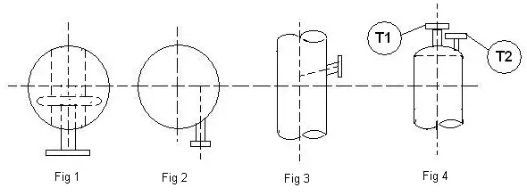
4. WRC 297 is not applicable for nozzles protruding inside the vessel (Fig 1), Tangential Nozzle (Fig 2), and Nozzle at an angle (Fig 3).
5. Typically, WRC-107 is used for local stress calculations and WRC-297 is used for flexibility calculations.
Fig. 1: Nozzles and Vessels for WRC
Limitations of WRC 107 (WRC 537) & WRC 297
Other than the boundary conditions mentioned above there are some more limitations as mentioned below:
Neither bulletin considers shell reinforcement nor do they address stress due to pressure.
CAESAR II, PVElite, & CodeCalc will not extrapolate data from the charts when the geometric limitations mentioned above are exceeded. Extrapolated data may not be appropriate.
WRC-107/ WRC-297 Calculation Methodology in Caesar II
Inputs required for performing WRC checking
The following documents must be ready with you before you start to perform WRC 107/297 checking:
Equipment Details/ General Arrangement Drawing
Nozzle details
Line list
WRC Calculation Steps in Caesar II
Step 1: Perform Static analysis of the stress system and find out the nozzle loads required for checking local stresses.
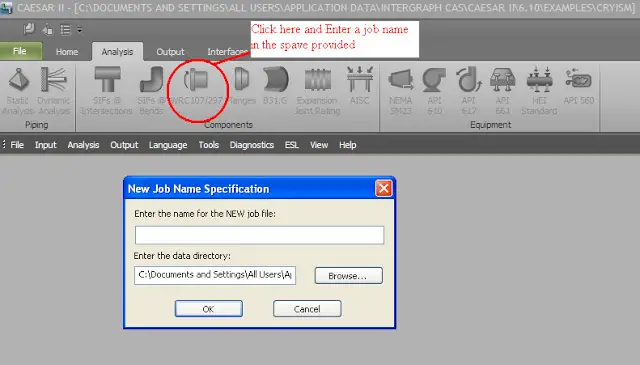
Step 2: Enter the WRC module from Caesar II. Provide a file name for your job. Refer to Fig. 2
Fig. 2: Opening WRC Module in Caesar II
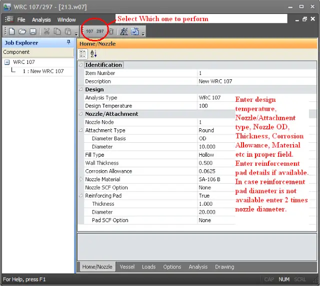
Step 3: The following screen will appear. Enter the Nozzle data as shown in Fig. 3 below.
Fig. 3: WRC Input Screen in Caesar II
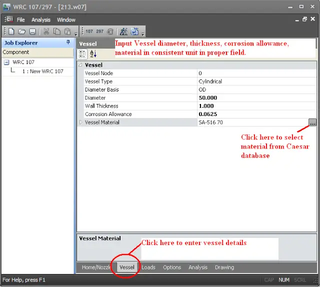
Step 4: Now enter the vessel details i.e, diameter, wall thickness, corrosion allowance, and material (Fig. 4)
Fig. 4: Input Vessel Details in Caesar II
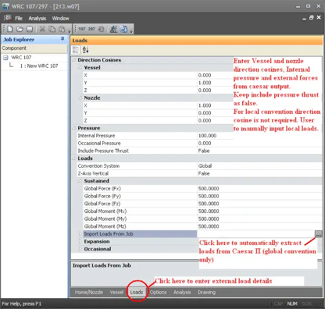
Step 5: Input vessel and Nozzle direction cosines, Internal design pressure, and load and moments values from Caesar static analysis output (Sustained, Expansion, and occasional as applicable).
Fig. 5: Entering Force Details
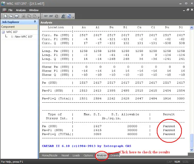
Step 6: On options, it is suggested not to change any parameter. Now click on analysis to read the results. The output will inform you whether WRC checking is passing or failing. Use results as per your requirements.
Fig. 6: Sample WRC Output Screen
For entering loads and moments as per local convention following description and figure (Fig. 7) can be used for converting global forces into local forces.
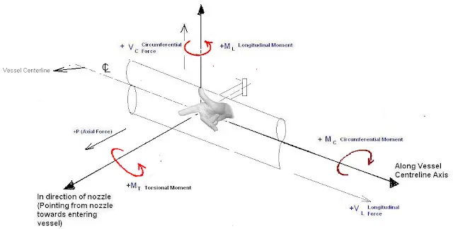
Fig. 7: Force and Moment Direction Consideration
As shown in Fig. 7, Stretch your right hand with the Middle finger along the Vessel Centerline. Index Finger should parallel to the nozzle centerline and should point in a direction from the nozzle towards entering the vessel. And the Thumb should be perpendicular to both. Then
The direction of the Index Finger represents +P.
The direction of the Middle Finger represents +VL
The direction of the Thumb represents +VC
ML will be positive if by applying the right-hand thumb rule to ML, the direction of thumb is the same as that of VC.
MC will be positive if by applying the right-hand thumb rule to MC, the direction of thumb is opposite to the direction of VL.
MT will be positive if by applying the right-hand thumb rule to MT, the direction of the thumb is opposite to the direction of P. Get the loads and moments from CAESAR output. Compare the direction of Forces and Moments in CAESAR output with conventional Force and Moment directions and enter the values of P, VL, VC, MT, MC, and ML accordingly.

