Recent Posts

What is Response Spectrum? | Steps for Earthquake Response Spectrum Analysis

A response spectrum is a graphical plot of the frequency of an oscillator and its damping. The response spectrum plot represents the peak or steady-state response (velocity, displacement, or acceleration) of a series of oscillators of varying natural frequencies. In the vibration analysis of any system, the response spectrum is very useful as the resulting plot can provide the response of any linear system with respect to its natural frequency. The response spectrum finds its usage in interpreting seismic or earthquake events and slug flow events.

Response Spectrum Analysis is a scientific method for estimating the structural response of dynamic vibration events. To perform the response spectrum analysis, the first job is to define the response spectrum of the system. In this article, we will explore the basics of the response spectrum and learn the steps for performing seismic/earthquake analysis using the response spectrum analysis method.

What is an earthquake?

Earthquakes are random ground motion that produces inertial loads in structures built on them. The ground motion of the earthquake can be attenuated by the building’s resonant response producing much larger motions at higher levels. That leads to major damage to the structure. Hence, structures need to be designed to withstand the earthquake’s ground motion.

Static vs Dynamic Seismic Analysis

This earthquake analysis of piping systems can be performed in two ways: by static method or dynamic way   

Static Equivalent Seismic Analysis:

Static equivalent analysis, for most non-critical piping systems, the earthquake is treated as a static load, which is proportional to the weight of the piping and components. The magnitude of the load is generally determined by the ‘g’ factor according to respective codes, for example, UBC, IBC, ASCE, IS, etc. This load is applied statically in the vertical and two horizontal directions.

Dynamic Earthquake Analysis

Dynamic Analysis, for critical piping systems, a dynamic analysis is generally preferred because that produces more realistic and accurate results compared to an equivalent static analysis. The random ground motion can be recorded using accelerometers and applied to the structure or piping model through all the ground supports as time histories and the effect can be assessed. These random ground motions are converted to response spectra to simplify earthquake analysis.

For seismic analysis of piping and structures, the earthquake response spectrum is the most popular tool. For predicting forces and displacements of pipes and structures, the response spectrum method provides various computational advantages. The main benefit of the seismic response spectrum method is the calculation of only the maximum displacement and force values in each mode of vibration using smooth design spectra that are the average of several earthquake motions.

Response Spectrum Analysis Method

Response spectrum plot gives the maximum response (that maybe maximum displacement, maximum velocity, maximum acceleration, or any other parameter of interest) to the natural frequency (or natural period) subjected to specified excitation for linear single-degree-of-freedom system oscillators. These plots are subjected to specific damping and it changes as damping changes. Refer to Fig. 1 shown below:

Definition of Response Spectrum
Fig. 1: Definition of Response Spectrum

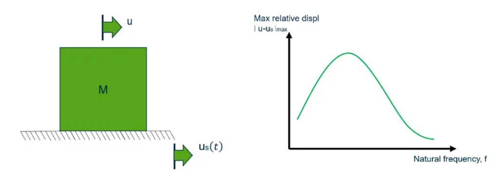
Here abscissa is the natural frequency (or period) of system and ordinate is the maximum response.

The plot of this type is shown here in the figure, in which a one-story building is subjected to a ground displacement indicated by us(t) and u indicates deflection.

For any linear single degree of freedom system, the response spectrum curve shown in the figure gives the maximum displacement of the mass m relative to the displacement at the support which is (us-u) here.

Example of Response Spectrum

Thus, to determine the maximum response of a linear single degree of freedom system from the available spectral chart, for specified earthquake excitation, one needs only to know the natural frequency of the system and damping.

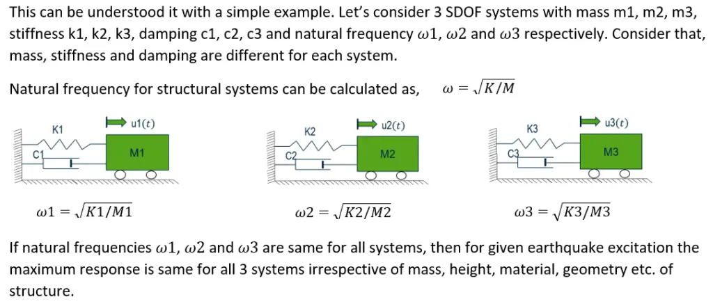
If the natural frequency of the structure coincides with the frequency of earthquake ground motion, it leads to a resonance condition, which creates substantial damage to the system. That’s the main reason, not all buildings collapse during an earthquake. The natural frequency of building/structure is a property of height, stiffness, material, etc. Buildings whose natural frequency matches with earthquake frequency collapse during an earthquake while remaining are not experiencing major damage.

The response spectrum is using the same principles as time history. Only instead of using time history, it is using maximum values of the response. When the time history profile is not available for a particular dynamic event, then the response spectrum is used. Response spectrum analysis provides more conservative results than time history.

Parameters affecting Response Spectra

The response spectral values are dependent on various factors like,

  • Soil condition
  • Energy release mechanism
  • Damping in the system
  • Epicentral distance
  • Focal depth
  • Richter magnitude
  • The time period of the system

Construction of Response Spectrum Plot

The construction of a Response Spectrum requires the solution of a single degree of freedom system, for a sequence of natural frequency values and damping ratio in the range of interest. Every solution provides only one point (with the maximum value) of the response spectrum. All of these maximum response values are plotted against natural frequency to construct a single response spectrum.

Since a large number of systems must be analyzed in order to fully plot each response spectrum, the task is lengthy and time-consuming. But once these curves are constructed and available for the excitation of interest, the analysis for the design of structure subjected to dynamic loading is reduced to a very simple calculation of the natural frequency of the system and the use of response spectrum to calculate the maximum response.

These response spectrum plots are created for specific areas of regions and different for different regions. The study of geographic areas combined with an assessment of historical earthquakes allows geologists to determine seismic risk and to create seismic hazard maps for respective areas, which show the likely maximum response values to be experienced in a region during an earthquake. 

So, let’s look at a simplified example of how we can get a response spectrum plot for a specific area of the region.

Constructing Response Spectrum Plot
Fig. 2: Constructing Response Spectrum Plot
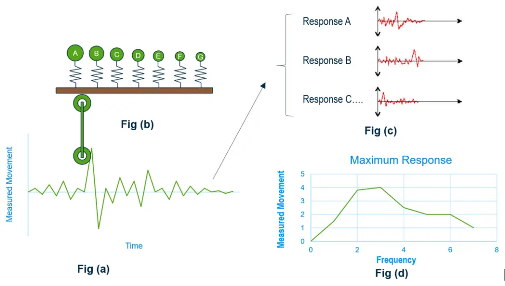
  • Step 1: First, take the randomly measured ground motion from previous earthquake records in that area. (Fig a)
  • Step 2: Then sequence of tuned SDOF oscillators with some fixed damping values attached to a shaker table and measured motion used to shake the table. (Fig b)
  • Step 3: The response of all the SDOF oscillators is recorded and plotted for an individual oscillator. (Fig c)
  • Step 4: Maximum response for all individual oscillators is extracted to plot the combined response. (Fig d)

Calculating the maximum response for a range of values of frequency and damping and then plotting results graphically to get a spectrum chart that shows the maximum response for all possible single-degree-of-freedom systems to that component of the earthquake. This maximum response can be maximum displacements, maximum velocity, or maximum acceleration. 

This combined response is made up of many peaks and troughs. The envelope of the broadened peaks is shown in fig (d), which is a conservative approach. The idea is that even though all earthquakes are different, the maximum response of similar earthquakes should be the same even though the time the maximum response occurs may differ i.e. timing of the event is not considered.

Seismic engineers and government planning departments use these values from the spectrum chart to determine the appropriate earthquake loading for buildings in the respective zone. Earthquake load impact calculations for any structure in that area of the region are simplified into a few steps to (a) calculate the natural frequency of the system, (b) and then the maximum response found from the respective spectrum chart for calculated natural frequency. 

Pseudo-acceleration and Pseudo-velocity

Response spectrum plots can be plotted as maximum relative displacement, maximum velocity, or maximum acceleration. These three quantities are also known as spectral displacement (SD), Spectral velocity (SV), and Spectral acceleration (SA) and are also proportional to each other.

The spectral displacement i.e. maximum relative displacement is proportional to spectral acceleration i.e. maximum absolute acceleration. This can be demonstrated with simple numerical iterations on the dynamic equation of motion.

Pseudo-acceleration and Pseudo-velocity

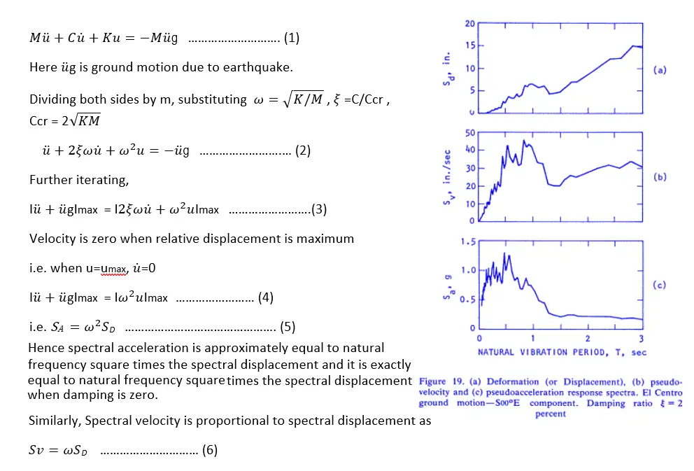
And this can be demonstrated by equating the equation for potential energy and kinetic energy.

The acceleration and velocity so defined are called pseudo-acceleration and pseudo-velocity, respectively. Pseudo-acceleration is very close to absolute acceleration and is the same as absolute acceleration when there is no damping. Pseudo-velocity is the fictitious velocity associated with the apparent harmonic motion for convenience.

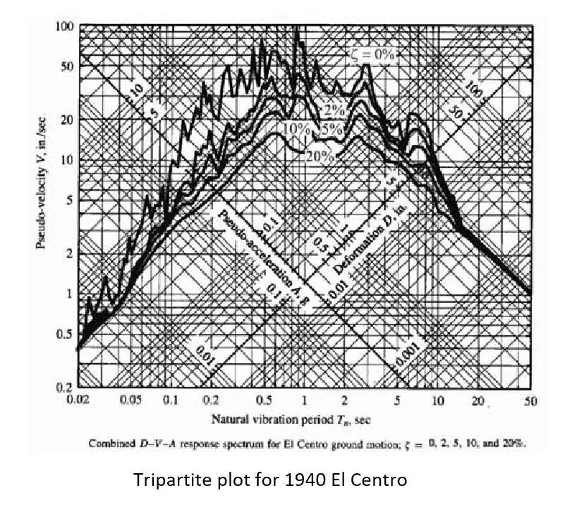
Tripartite Response Spectra

It is possible to plot all three responses in a single chart using a logarithmic scale and it is called the Tripartite plot (Fig. 3)

Sample Tripartite Plot
Fig. 3: Sample Tripartite Plot

Dynamic Equation of Motion and Modal Superposition

The dynamic behavior of a piping system depends greatly on the free or natural vibration of the system. SDOF system deals with one natural frequency and this system can only move in one particular direction. However, in a multi-degree of freedom (MDOF) structural system, such as a piping system, there are many natural frequencies, each with its vibration shape or mode. These MDOF structures with N degrees of freedom system transformed into the problem of solving N systems, in which each one is an SDOF system. This transformation extends the use of response spectra from a single-degree-of-freedom system to the solution of the system with any number of degrees of freedom.

The equation of dynamic equilibrium associated with the response of the structure subjected to ground motion is as below.

Equations for Response Spectrum

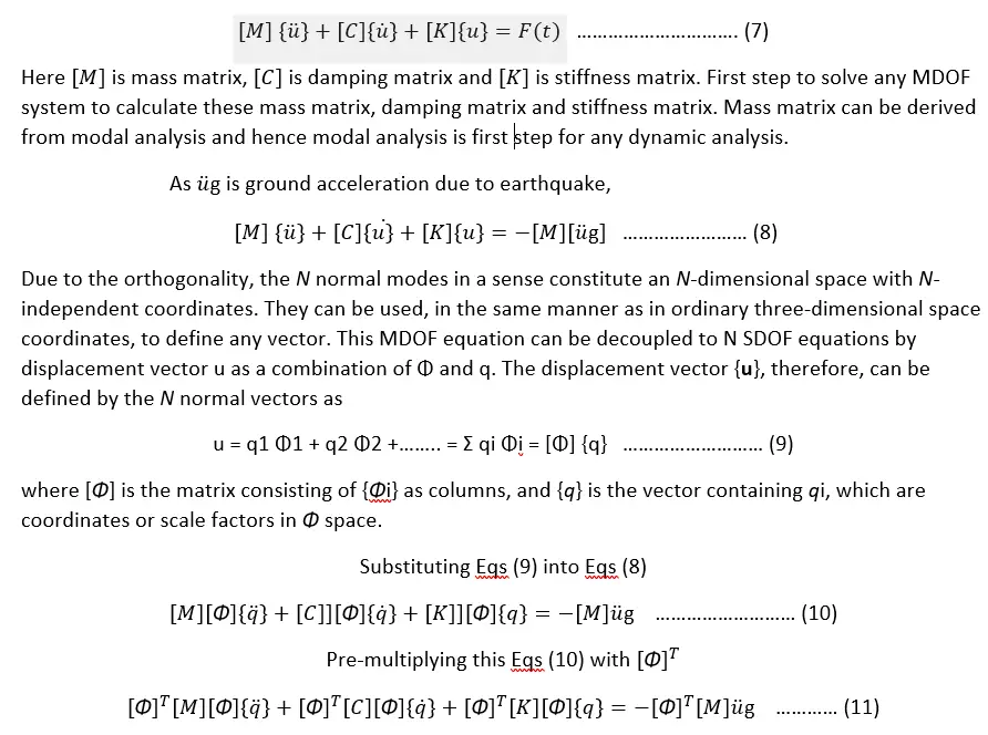
Due to modal orthogonality, M, C, and K matrices will become diagonal matrices. The modal superposition converts the N simultaneous differential equations of the MDOF system into N-independent SDOF systems by decoupling this equation. These N-independent SDOF systems are solved one by one using SDOF techniques.

Response Spectrum Equations 2

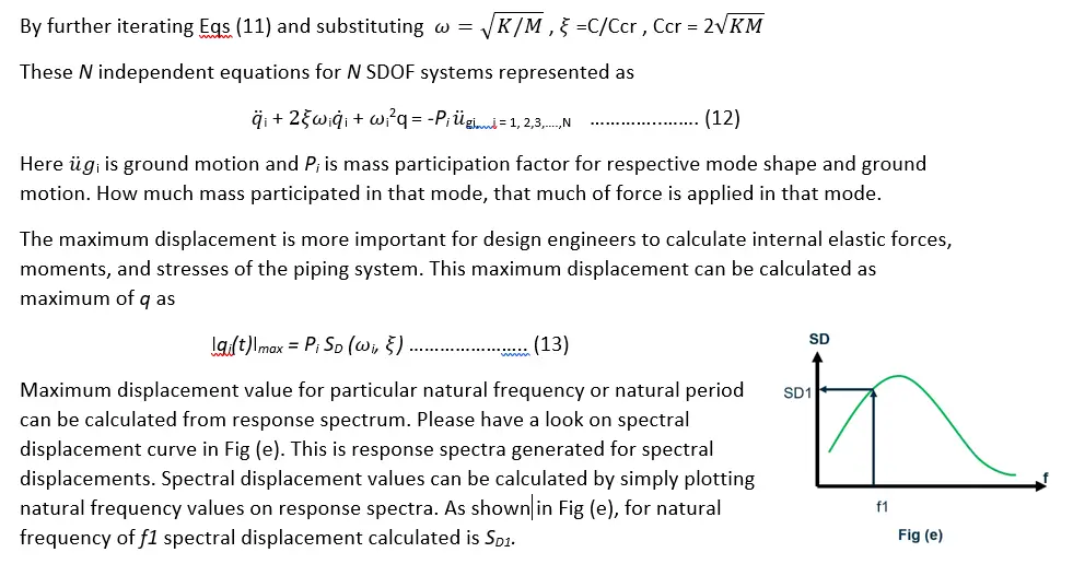
The maximum displacement in time history response can be calculated by multiplying the maximum displacement calculated from the response spectrum with the participation factor for the respective mode shape. Each mode shape is contributing up to some extend to the total response of the structure and that depends on the participation factor. Accordingly, the maximum response is calculated for all respective modes.

The amount of displacement in one mode given by,

Equation 14

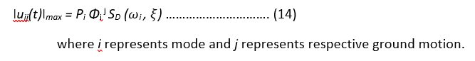
Accordingly, the maximum time history response is calculated for all modes and respective ground motions and combined together to get maximum earthquake response. These maximum time history responses cannot be added directly and for that special techniques called modal combinations are used.

Modal Combinations

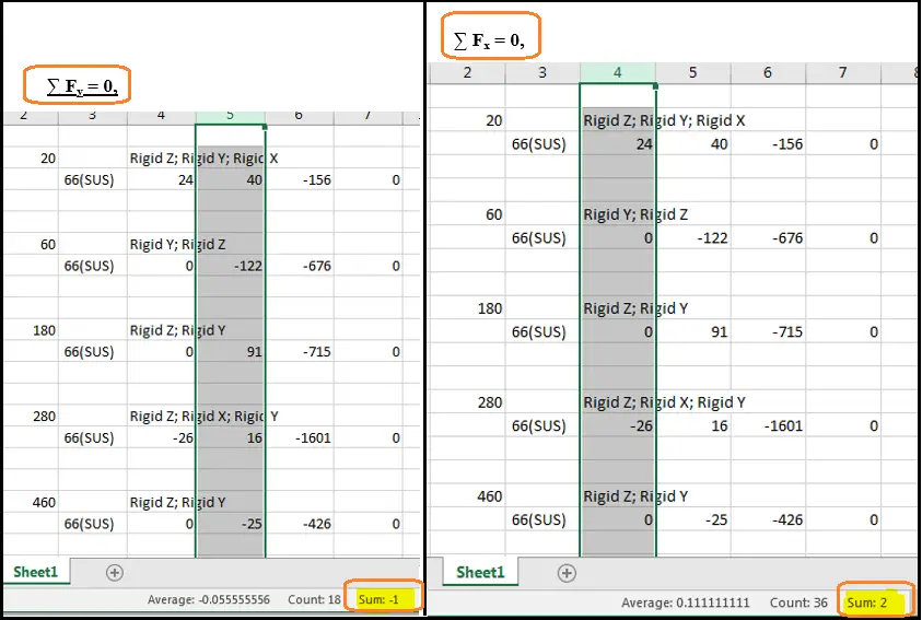
The total response of the system is determined by combining the responses from all modes. This combination is termed a modal combination. The modal combination includes internal modal forces and internal modal moments, as well as modal displacements.

Ed Wilson and Ray Clough took the response spectra method and developed the approximate method for MDOF structures that requires the combination of the modes and proposed SRSS over 50 years ago.  At that time only 3 earthquake records existed for comparison whereas now we have thousands.

The methods of combining modal results present some confusion to many piping engineers. We have the SRSS (Square Root of Sum of Square), ABS (Absolute), CQC (Complete Quadratic Combination), and a few algebraic methods. They all have been used in one situation or another. However, we do not really have a clear picture of when and why a certain method is used.

The NRC Regulatory Guide 1.92 provides further guidance for nuclear facilities. Some of the methods are from Rev 1 and some are from Rev 2 with some standard mathematical methods.

  • Square Root of the Sum of the Squares (SRSS)
  • Grouping Method
  • Ten Percent Method
  • Absolute Double Sum Method
  • Signed Double Sum Method
  • Absolute CQC
  • Signed CQC

Steps to perform Response Spectrum analysis in AutoPIPE

  • Open Model in AutoPIPE from, File>Open.  Note: The first step for any Dynamic analysis is modal analysis.
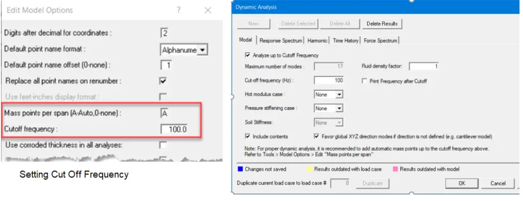
  • Go to Tools > Edit Option and make these changes:
    • Mass point per span (A-Auto, 0-None): A
    • Cutoff frequency: 100
  • Then click OK to accept.

Note: Specifying ‘A’ means that the mass spacing will be applied automatically using a frequency of 100Hz. It is possible to split each length into the same number of spans by using a number in the range 1-9 instead of A, but this can lead to very closely spaced nodes in short lengths.

  • Go to Analysis > Dynamic analysis to set up dynamic analysis settings
  • Under Modal analysis, check on Analyze up to Cutoff frequency and Provide cutoff frequency value. Review other information if you want to make modifications over there. And then click OK
Response Spectrum Analysis Steps in AutoPipe
Fig. 4: Response Spectrum Analysis Steps in AutoPipe

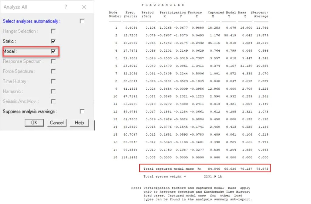
Then click on Analyze all from the Analysis ribbon. Make sure that Modal analysis is selected and click ‘OK’.

Check for adequate mass participation. Go to Result > Output Report, select Frequency report and click ‘OK’ to access reports.

Response Spectrum Frequencies
Fig. 5: Response Spectrum Frequencies

The next step is to create a Response spectrum. Go to Loads>Response Spectrum. Here you can provide a new Response Spectrum Or can use an existing one.

Response Spectrum Generation in AutoPIPE
Fig. 6: Response Spectrum Generation in AutoPIPE

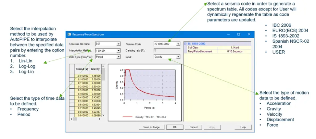
Note: You can provide a number of response spectra together. This spectrum data can be copy pasted from MS Excel. Also, you can construct spectrum may as an external ASCII text file using any text editor software.

  • Now go to Analysis>Dynamic analysis>Response Spectrum.
  • Create a new load case by clicking on ‘New’. Then click on Spectra>Define.
New Response Spectrum Generation
Fig. 7: New Response Spectrum Generation

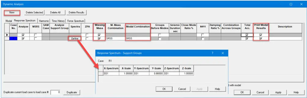
Missing mass correction can be considered by checking on ZPA or Missing Mass field. Then from the dropdown select Modal Combination type for calculations. Check on ‘Print Modal Results’ and click ‘OK’.

Note: Different Response spectra can be provided for each direction. Also, scale factors can be modified.

  • To analyze the model for Response Spectrum, click on Analyze All in the Analysis ribbon. Please make sure the Response Spectrum is selected here.
  • After analysis, Go to Result>Combinations.
  • A new load case is created for Response Spectrum, Response 1 (R1)
Response Spectrum Load combinations
Fig. 8: Response Spectrum Load combinations

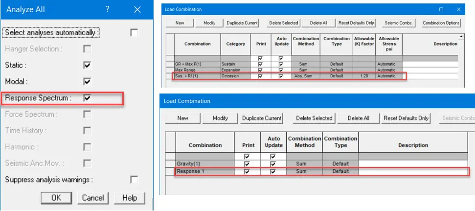
Code Combinations are used to check code stresses whereas Non-Code Combinations are to check forces and moments. Code combination Sus+R1 and Non-code combination R1 are created automatically by AutoPIPE. This R1 we can further combine with other operating cases.

  • These results can also be checked graphically,
  • Code stresses,  Go to Result>Code Stresses, and then select Sus+R1 as combinations.
  • Displacements, Go to Result>Displacement and then select Response 1 as Load combination.
  • Detailed text reports for Response, Mode Shapes, Restraint Reactions, and Accelerations can get from Quick reports.
  • Go to Result>Quick Reports>Output Report and select Frequency, Mode Shapes, Restraint, and Accelerations.

Results and Interpretations of Response Spectrum Analysis Outputs

This maximum response can be found from provided response spectrum and modal analysis results as explained in the Dynamic Equation of Motion and Modal Superposition theory.

Modal analysis results provide different modes of natural frequency and participation factors.

Output result of Response Spectrum in AutoPipe
Fig. 9: Output result of Response Spectrum in AutoPipe

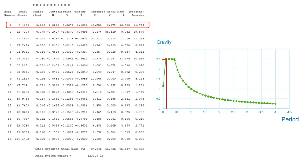
By simply, plotting the period (or natural frequency) value on spectra, the maximum response is calculated. This maximum response is multiplied by the participation factor to calculate the maximum time history response in the respective mode. Accordingly, maximum responses are calculated for all modes and combined by Modal combinations to get a maximum response due to earthquake loading at all points.

About the Author: This article is prepared by Mr. Manoj Kale, AutoPipe Expert. He presented this article in the form of a webinar. To access the recording of that webinar and learn directly from the expert, Click here and register.

What is Piping Fabrication? | Tools for Pipe Fabrication

Pipe fabrication can be defined as the process of cutting, bevelling, and welding piping components such as pipes, tees, elbows, flanges, reducers, etc., as dictated by the design documents. In the process and power piping industry, Piping fabrication is a highly critical activity as it involves hundreds of components and thousands of steps and requires a high degree of precision. In any construction project wherever piping networks are involved, piping fabrication needs to be properly planned, scheduled, and executed as per design requirements. To maintain the system integrity, and proper functioning of each item, and minimize accidents, It is required to ensure maximum quality of work during pipe fabrication. In this article, we will explore more details about piping fabrication.

Piping fabrication involves various activities like piping material storage and handling, cleaning, cutting, bevelling, welding, inspection and testing, painting, insulation installation, etc.

Types of Piping fabrication

Depending on the location of the pipe fabrication work they are classified into two groups.

  • Shop Pipe Fabrication and
  • Field Pipe Fabrication.

Shop Fabrication vs Field Fabrication

There are various factors that determine whether pipes will be shop fabricated or field fabricated or both methods will be used. In most cases, both shop and field pipe fabrication is used. The major deciding factors are profitability, type, and size of the project, piping material, and size, post-fabrication surface treatment, environmental condition, accessibility of equipment, skilled personnel availability, time requirement, and availability, etc.

In general practice, small bore pipes, threaded and socket welded pipes are field fabricated whereas butt welded pipes, pipe bending, modular items, etc are shop fabricated.

In the Shop pipe fabrication process pipe, fittings and components are assembled by welding into spool assemblies at the fabricator’s facility or a workshop normally known as a pipe fabrication shop. The spools are then labeled using an identifier and transported to the construction site for installation. Whereas in field pipe fabrication all these assemblies are done at the construction site.

Tools/Equipment used for Pipe Fabrication

During pipe fabrication, various equipment and tools are used that helps in the fabrication process. The widely used equipment is listed below:

  • Pipe Jacks
  • Adjustable Pipe Rollers
  • Welding Machine
  • Pipe Rigging and transport equipment
  • Chain Clamps/ C Clamps
  • Pipe Fit-up Tools
  • Pipe Purging Equipment
  • Pipe Cutting and Bevelling Equipment
  • Torque Wrench/Adjustable Wrench/Combination Wrench/Hammer Wrench
  • Flange Alignment Tools and Pins
  • Center Punch
  • Compass/Contour Marker
  • Pipe Threader
  • Fork Lift
  • Grinder
  • Wraparound Tapes
  • Hydraulic Crane/Tower Crane
  • Pipe Bending Machine, etc
Typical Pipe Fabrication tools

Preparation for Pipe fabrication

In this stage, pipe fabricators are required to calculate various parameters from the drawing specifications. They are required to take into consideration welding and tack welding processes along with any distortion that may arise from welding. The tools required for the fitting-up of pipes and flanges, such as pipe supports and clamps will also need some thought. Then they need to prepare a simple wire model of the pipe spool from the drawings. Material take-off and the client’s fabrication specification are also supplied to the pipe fabricators.

Pipe fabrication in a Pipe fabrication Shop
Pipe fabrication in a Pipe Fabrication Shop

Piping Fabrication Procedure

The pipe fabrication process requires assembling pipes and pipe fittings according to the spool drawing. Pipe fabricators must take into consideration the size of the assembly, as transportation could be a problem. In such cases, Sub-assemblies are an effective way of transporting large projects. Piping fabrication is done as per the below-mentioned steps:

  • Marking and Cutting: As per the design drawing requirement, Marking shall be done and the same shall be verified by the concerned supervisor prior to cutting. Pipe cutting is normally done as follows:
    • Carbon Steel pipes – By gas cutting & grinding.
    • Alloy Steel pipes – By grinding or flammable cutting.
    • Stainless Steel Pipes – By grinding or plasma cutting.
  • Tagging: Using dye stamping, Paint marking, or Tagging, pipe heat numbers are transferred to the cut pieces before cutting the pipe.
  • End Preparation: In the next step, End preparation (bevelling) and fit-up are done following an approved Specification and WPS.
  • Welding Pipes: Extra precautions must be exercised to ensure that longitudinal seams on the joining pipes do not come in one line in a butt-welded joint. Seams must be staggered at least 100 mm apart and also will clear the branch connections. Care is taken to make sure that longitudinal seams are not resting on the steel structure.
  • Welding Pipes and Fittings: Pipes and Fittings for fit-up are then placed on a temporary pipe bed and supports are properly secured properly. Next, the arrangement is inspected for quality Fit-Up. Once inspection clearance is received, Joints are welded by qualified welders.
  • Details Marking: Various details line pipeline No., Component Heat No., Joint No., Fit-up inspection signature, Welder No., Visual inspection signature, and welding date are marked near the joint using a metal paint marker.
    • The pipe Spool Number is marked with a paint marker and an aluminum tag is tied to the spool.
  • Heat treatment: As per project-specific requirements, Preheating and PWHT will be done at the shop or field.
  • Fabricated pipe spools are then shifted from the pipe fabrication shop to the laydown area.
  • Inspection: As per the requirement of the project specification or guidelines, NDT is performed. Once NDT clearance is received, spools are released for erection/painting with a release notice.
    • Spools rejected in the NDT process are identified with yellow and black tags and sent for repair work. NDT has performed again on the repaired weld areas as required.
  • Documentation: After painting, field inspection is executed for QC and the same is recorded in the prescribed format. After the painting inspection, the spool is released for erection.
  • Fabrication of Stainless Steel Pipes: Stainless Steel piping fabrication is normally done in the shop with an isolated area from carbon steel and alloy steel. The equipment and tools which are used for CS fabrication shall not be used for SS. Tools for SS must be differentiated clearly by marking “For Stainless Steel” only. For Stainless steel materials, stainless steel tools will be used for grinding, brushing and clamping, etc.
  • Protection: For the protection and temporary storage till the erection, all flanged raised faces of completed pipe spools are fitted with plywood blinds and spool ends shall be fitted with proper caps.

Pipe Fabrication Shop

The pipe fabrication Shop is basically a workshop where all the prefabricated pipe spools are developed. All the pipe works for spool preparation are normally performed inside this shop using highly skilled pipe fabricators. Generating pipe spools in the Pipe Fabrication shops is the best economic way for reducing site installation costs for big-size projects. All equipment, tools, and manpower are available in the pipe fabrication shop and pipe spools are produced with high quality.

Pipe Fabrication Specification

Pipe fabrication Specification is an engineering document that provides all guidelines to be followed by pipe fabricators for spool pipe fabrication. The specification for piping fabrication provides the minimum requirement of preparation of detail shop drawings and the fabrication, requirements for inspection and testing. It lists all applicable codes and standards.

15 Most Common Welding Defects, Causes and Remedies

Welding defects can be defined as unacceptable imperfections during the welding process. Any unacceptable deviation with respect to set technical and design requirements in the welding process is termed as welding defects. Various parameters could cause deviation from the ideal welding process as defined by the codes and standards. Wrong welding, human behavior, wrong electrode, poor process condition, improper job preparation, unskilled welder, incorrect weld parameters, etc could be some of such reasons. Defects in Welding can occur at any stage of the welding process and they can easily be detected in form of geometric imperfections. Such weld defects can affect both the inside and outside of the metallic structure.

Various codes and standards like BS EN ISO 6520-1, BS EN ISO 5817, and BS EN ISO 10042 provide acceptable limits for welding irregularities. When any discontinuity exceeds those acceptable code limits they are considered welding defects. It is important that a welding defect is correctly identified so the cause can be established and actions are taken to prevent further occurrence.

Types of Welding Defects / Welding Defect Types

Depending on the location of the Welding defects, they are classified into two groups:

  • External Welding Defects and
  • Internal Welding Defects.

External welding defects are found on the surface itself and can sometimes be recognized by the naked eye. Surface Cracks, Undercut, Porosity, Overlaps, Craters, Underfill, Spatters, Excessive penetration, Arc Strikes, etc are examples of external welding defects.

Internal welding defects exist in the material at some depth and are hidden from the naked eye. Incomplete penetration, Slag inclusion, Internal porosity, Internal crack, Incomplete fusion, Internal Blowholes, etc are examples of internal welding defects.

In the welding process, both internal and external types of welding defects are quite common. In the next paragraphs, we will explore these types of welding defects in detail.

Welding Defects Crack

Welding defects Crack is an imperfection produced by a local rupture in the solid state arising from the effect of cooling or stresses. Welding Cracks are more significant than other types of welding defects as their geometry produces a very large stress concentration at the crack tip making them prone to cause a fracture.

Welding cracks are normally found in the weld metal, parent metal, or the Heat Affected Zone. Welding Defect cracks can be of various types like:

  • Longitudinal.
  • Transverse.
  • Radiating.
  • Crater (found only in the weld metal)
  • Branching.

Welding defect cracks can be of various shapes and sizes and may appear on the surface or at any depth or even at the root. The main reason for the crack is the localized stress exceeds the UTS of that material.

Depending on their nature, these welding cracks can be:

  • Hot cracks
  • Cold cracks
  • Lamellar tearing.

Hot Cracks:

Hot cracks normally occur during the solidification stage; which means soon after welding. Depending on their location and mode of occurrence, hot cracks can be of two types:

  • Solidification cracks: They occur in the weld metal during the solidification process.
  • Liquation cracks: They occur in the coarse grain HAZ, as a result of elevated temperature heating of the material that causes liquation of the low melting point constituents on the grain boundaries.
Welding Defects-Solidification Hot Crack
Fig. 1: Welding Defects-Solidification Hot Crack

Solidification cracking (Fig. 1) normally occurs when:

  • Weld metal possesses high carbon or impurity content.
  • The solidifying weld bead has a larger depth-to-width ratio (deep and narrow).
  • Heat Flow disruption occurs.

The cracks can be wide and open and possibly narrow. Solidification cracking occurs in compositions having a wide freezing temperature range. For steels, solidification cracks occur due to the presence of high carbon content and impurity elements like sulfur and phosphorus. During solidification, these elements segregate such that intergranular liquid films remain once the bulk of the weld has solidified. The thermal shrinkage of the cooling weld bead can cause these to rupture and form a crack.

Cold Cracks:

Cold cracks occur after the weld metal solidification in the grain-coarsened region of the HAZ. They are also known as delayed cracking as they can normally develop after several days of welding. It lies parallel to the fusion boundary and its path is usually a combination of inter and transgranular cracking.

The direction of the principal residual tensile stress can result in the cracks causing the crack path to grow progressively away from the fusion boundary towards a region of lower sensitivity to hydrogen cracking. When this happens, the crack growth rate decreases and eventually arrests.

Welding Defects-Cold Crack
Fig. 2: Welding Defects-Cold Crack

The main causes of Cold cracks (Fig. 2) are Lack of preheating, Low temperature, high stresses, susceptible material structure, high hydrogen content, etc.

Lamellar tearing:

Lamellar tearing normally occurs in rolled steel plates. They are distinguished by the cracking feature having a terraced appearance. Lamellar Cracking occurs in joints where:

  • A thermal contraction strain can occur in the through-thickness direction of the steel plate.
  • The possibility of non-metallic inclusions as very thin platelets with their principal planes parallel to the plate surface is high.
Welding Defect-Lamellar tearing
Fig. 3: Welding Defect-Lamellar tearing

Welding Defects Undercut

Undercuts are welding defects that present themselves as irregular narrow grooves on the parent metal. They are characterized by their depth, length, and sharpness. The undercut runs parallel to the weld metal and acts as a stress raiser during fatigue loading due to the weakened section. Welding defects Undercut is of three types; Continuous undercut, Intermediate undercut, and Inter-run undercut.

Causes of Undercuts

Probable causes of undercut welding defects are

  • Melting of the top edge due to fast weld speed or high voltage.
  • High arc voltage.
  • Too large electrode; Incorrect electrode angle.
  • Use of wrong filler metal.
  • Incorrect shielding gas selection.
  • Excessive weaving
Welding Defect-Undercut
Fig. 4: Welding Defect-Undercut

Remedies/Prevention of Welding undercut

The following steps should be exercised to prevent the possibility of undercut welding defects.

  • Decrease the travel speed, Reduce the power input.
  • Use the right electrode size with correct positioning; between 30 to 45 degrees angle.
  • Reduce the length of the arc and lower the voltage.
  • Weld in flat positions.
  • Use proper current with attention to thinner areas and edges.
  • Use the correct gas mixture based on material type and thickness.

Heat input must be controlled during weld repairs of undercut welding defects.

Welding Defects Porosity

Welding Defect Porosity is caused by the entrapment of gas or air bubbles in the weld metal. These trapped gases collapse over time and weaken the weld section. They can be localized or uniformly distributed. Depending on the Porosity formations they are of various types:

  • Gas Porosity
  • Worm Holes
  • Surface Porosity

Gas Porosity:

Gas porosity is a small cavity of spherical shape generated in the weld metal due to the trapped gases. They are of various forms like Isolated; Uniformly distributed porosity, Surface pore, Localized Clustered porosity; Elongated cavity, or Linear porosity.

Worm Holes:

Sometimes, during solidification, the trapped gas can form tubular or elongated cavities which are known as Wormholes. They can appear singly or in groups over the weld surface. Progressive entrapment of gas between the solidifying metal crystals causes wormholes.

Surface Porosity:

Porosities that break the surface are known as surface porosities. They are similar to uniform porosities.

Welding Defect-Porosity
Fig. 5: Welding Defects-Porosity

Causes of Porosity

Major causes of welding defect porosity are:

  • The electrode is not well coated / Corroded Electrode
  • Presence of oil, grease, hydrocarbon, water, or rust on the weld surface.
  • Use of incorrect shielding gas or improper shielding or air entrapment.
  • Too high gas flow/ Too great arc voltage
  • Gas evolution due to improper surface treatment.

Prevention or Remedies of Porosity:

To reduce the formation of welding defect porosity the following remedial actions can be taken:

  • Clean the weld surface and materials; Ensure that the prepared surface is free from oil, rust, or other contaminants.
  • Use of dry, good-quality electrodes.
  • Optimize the welding process to allow gases to escape.
  • The gas flow meter is to be configured with the correct flow settings.

Welding Defects Overlap

Welding defect overlap occurs when the weld pool overflows on the welding surface of the parent metal. In such a scenario, the molten metal does not fuse with the base metal.

Causes of Overlaps:

  • Large weld deposition in one go.
  • Poor electrode manipulation; Wrong electrode coating.
  • Using the electrode at the wrong angle.
  • High current/Heat Input.
  • Incorrect Weld positioning.
  • Longer arc.
Welding Defect-Overlap
Fig. 6: Welding Defects-Overlap

Remedies of Overlap:

  • Use the correct welding technique to avoid the wrong arc length.
  • Position the electrode at the appropriate angle.
  • Change to a flat position.
  • Use correct deposition during each run; Correct Electrode Coating
  • Use low welding current; Low heat input.

Welding Defects Solid Inclusions

Various solid particles may be included during the welding process. These welding defects are known as solid inclusions. They can be of various types as listed below:

  • Slag inclusion
  • Oxide inclusion
  • Flux inclusion
  • Metallic inclusion
    • Tungsten
    • Copper
    • Other Metal
Welding Defect-Slag Inclusion
Fig. 7: Welding Defects-Slag Inclusion

Welding Defect Lack of Fusion

Welding defect lack of fusion arises due to incomplete fusion between the weld metal with the parent metal. Lack of fusion is also known as Cold lapping or cold shuts. Lack of fusion is an internal welding defect, but it can occur on the external surface too. Lack of fusion can be categorized into three groups:

  • Lack of sidewall fusion
  • Lack of inter-run fusion and
  • Lack of root fusion
Welding Defect-Lack of Fusion
Fig. 8: Welding Defects-Lack of Fusion

Causes for welding defect Incomplete or Lack of fusion:

The following parameters can contribute to the lack of fusion welding defects:

  • Low heat input/Low Arc current
  • Wrong electrode diameter with respect to the material thickness.
  • High travel speed.
  • Large Weld Pool.
  • Improper bead placement.
  • Oxide or Scale in weld preparation.
  • Large Root Face/Small root gap/Excessive root misalignment

Remedies/Prevention of Lack Of Fusion:

To prevent or reduce the possibility of incomplete fusion the following steps can be followed:

  • Reduce travel speed.
  • Appropriate bead positioning.
  • Maintaining Correct root gaps.
  • Increase current or heat input.
  • Inprove edge preparation.

Welding Defect Lack of Penetration

When the weld metal doesn’t completely penetrate the joint, It creates the weld defect known as lack of penetration or incomplete penetration. As the weld depth is not sufficient, this zone will be highly stressed and can fail easily. They are of two types; Incomplete penetration and Incomplete root Penetration.

Welding Defects-Lack of Penetration
Fig. 9: Welding Defects-Lack of Penetration

Causes behind Lack of Penetration welding defects:

  • Excessive thick root face.
  • Root gap is too small
  • Fast travel speed
  • Use of vertically down welding
  • Low heat input
  • Too large electrode

Prevention of welding defect Incomplete Penetration:

  • Reduce Electrode Size
  • Proper joint preparation i.e. providing a suitable root gap.
  • Proper heat input
  • Correct travel speed
  • Vertical up procedure

Welding Defects Spatter

Spatters as welding defects are small globular weld metal droplets expelled during the welding process and stuck to the base metal surface.

Reasons For Spatter:

  • High Welding current can cause this defect.
  • Damp Electrodes.
  • The longer the arc the more chances of getting this defect.
  • Magnetic Arc Blow.
  • Incorrect polarity.
  • Improper gas shields may also cause this defect.
Welding Defects-Spatter
Fig. 10: Welding Defects-Spatter

Remedies for Spatter:

  • Reduce the arc length and welding current
  • Use dry electrodes.
  • Using the right polarity and according to the conditions of the welding.
  • Use of AC power.
  • Increasing the plate angle and using proper gas shielding.

However, Spatter does not affect the weld integrity and can be easily removed by brushes.

Welding Defects Distortion

The excessive heat during the welding process creates distortion. This welding defect is usually found on thinner welding plates where the surface area is not sufficient to dissipate the heat. Due to excess heat, the shape gets changed and hence the name distortion.

Causes of Distortion:

The common causes of distortion are:

  • Varying temperature gradient.
  • Thin weld plate
  • Slow arc travel speed
  • A large number of weld pass

How to Prevent Weld Distortion?

  • Using a weldable metal type.
  • Optimizing the number of weld passes.
  • Suitable welding method depending on the metal.

Welding Defect Arc Strike

Arc Strike is usually caused by improper workmanship. When a welder accidentally strikes the electrode or the electrode holder against the work, unwanted arcs are generated adjacent to the weld. These spots are known as “arc strikes” which can initiate failure during bending or cyclic loading.

Remedies: Care must be exercised during welding. The repair can be done by chipping.

Welding Defect Burn Through

Burn-through creates holes in the parent metal.

Causes:

  • Excessive root gap
  • Excessive weld current
  • Insufficient root face

Remedies:

  • Keeping proper root gap.
  • Controlling the weld current.
  • Can be repaired by removing the hole and re-weld and then PWHT

Welding Defect Convex and Concave Weld

This type of welding defect is characterized by misshaped welds; usually convex or concave shapes. The main reason that causes convex and concave welding defects are welding using incorrect speed and electrode current. Using optimal welding current and proper electrode size this type of weld defect can be prevented from occurring.

Welding Defects Excessive Penetration

Excessive penetration is a type of welding defect generated due to high penetration through the joints. It creates notches on the weld surface where high-stress concentration takes place.

Welding Defects Blow Holes

When the generated gas during welding can not escape before molten metal solidification, this type of weld defects form. They are characterized by spherical cavities inside the bead. This is a surface defect.

Welding Defect Shrinkage Cavity

This is the cavity formed by the weld metal shrinkage during solidification.

Other Welding defects

There are some other welding defects as mentioned below:

  • Warpage
  • Excess weld Metal
  • Linear Misalignment
  • Irregular Width
  • Root Concavity
  • Stray Arc
  • Torn Surface
  • Incorrect profile
  • Grinding Mark
  • Under-flushing
  • Chipping Mark, etc

Fig. 11 shows a few of those welding defects.

Various Welding Defects
Fig. 11: Various Welding defects

Few more welding articles for you.

Welding Galvanized Steel
Overview of Pipeline Welding
Welding Positions: Pipe Welding Positions
Welding Defects: Defects in Welding: Types of Welding Defects
Welding Inspector: CSWIP and AWS-CWI
General requirements for Field Welding
Underwater Welding & Inspection Overview
Methods for Welding Stainless Steel

Weld Acceptance Criteria for Completed Welds

To understand the acceptance criteria for completed welds, one should refer to the governing welding code and standards. For example, Table 341.3.2 of ASME B31.3 (Fig. 12) provides the Acceptance Criteria for welding for Process Piping. For pressure vessels, the acceptance criteria for welding are provided in ASME BPVC Section VIII, Div 1.

Acceptance Criteria for Welds
Fig. 12: Acceptance Criteria for Welds as per ASME B31.3

However, in general, the following points should be noted for the acceptance criteria of piping welds:

  • Crack is not permitted.
  • Weld surfaces free from overlaps, abrupt ridges, and valleys are permitted.
  • Reinforcement thickness shall not exceed 3/16 inches.
  • Undercuts shall not exceed 1/32 in. or 12.5% of the wall thickness whichever is less.
  • In the case of single-welded joints, the concavity of the weld root surface should not reduce the total joint thickness (including reinforcement), to less than the nominal thickness of the thinner component being joined.
  • For single welded joints, the excess root penetration shall exceed the lesser of 1/8 in. or 5 % of the pipe inside diameter.
  • Incomplete root penetration is acceptable if it does not exceed the lesser of 1/32 in. or 20 % of the required thickness, and its extent is not more than 1 ½ in. in any 6 in. lengths of the weld.
  • The length of unfused bead or layer areas shall not exceed 20 % of the pipe circumference, or of the total length of the weld, and no more than 1½ inches in any 6 in. lengths of the weld.

Online Welding Courses

To enhance your knowledge regarding welding, the following video courses can be undertaken:

Types of Pipe Fittings and Components for Piping, Pipeline, and Plumbing Industry

Pipe Fittings are defined as the piping components that help in pipe routing for directional changes, size changes, and branch connections. Piping Elbows, Piping Reducers, Tee Connections, Olet Connections, Caps, Crosses, etc are pipe fittings and are widely used in both the piping and plumbing industries. Different pipe fittings serve different functions as per layout or process requirements. Pipe fittings are manufactured as separate items and procured separately. Pipe fittings are connected to piping using various end connections. Pipe fittings play an important role in the proper functioning of pipes and tubes in various applications. In this article, we will study the overview of different types of pipe fittings used in the piping, pipeline, and plumbing industry.

Types of Pipe Fittings

Various types of pipe fitting are used in piping, plumbing, and pipeline industries to serve as branch connections or other inline piping components. Common Pipe Fittings that are widely used in industries are listed below.

However, note that if a pipe or pipeline is bent at a pipe fabrication shop to change the direction it is not a pipe fitting. Pipe fittings are always separate items from the pipe. Click on the Bold and italics words above to know about those items in detail as I had already published separate articles on those. We will discuss the remaining pipe fittings in the next paragraphs.

The following image (Fig. 1) shows various types of fittings for reference.

Pipe fittings for Piping and Plumbing Industries
Fig. 1: Pipe fittings for Piping and Plumbing Industries

Pipe Union/Pipe Fitting Union/Pipe Union Fitting

Pipe Union is a special type of pipe fitting that unites two pipes and can be easily detached without any deformation to the pipes. They provide a positive seal and easy assembly as well as disassembly. In pipe fitting applications, They are widely used mainly for small bore piping and plumbing industries. Pipe unions are made of Carbon steel, Stainless steel, Cast iron, Copper, Nickel, Aluminum, Plastic, and Alloy materials depending on temperature, and service requirements.

A pipe union has three parts; A male end, A nut, and a female end. The female end has threads on the inside whereas threads are outside on the male end part. The nut provides the necessary pressure and seals the joint. Fig. 2 represents typical pipe unions used in the pipe fitting industry.

Pipe Unions
Fig. 2: Pipe Unions

Pipe Adapters

Adapters as pipe fittings are used to connect dissimilar pipes. Pipe adapters are available in various types for different applications. So care must be exercised while ordering to get the right type. They are classified as Locking Pipe Adapters, Offset Pipe Adapters, Male Pipe Adapters, Female pipe Adapters, Straight Thread adapters, etc. They find their majority of applications in sanitary pipes for plumbing applications. Normally they are made of Steel, Cast iron, polymers, Brass, Aluminum, Bronze, and copper materials.

Pipe Adapters
Fig. 3: Pipe Adapters

Pipe Olet Connections

Piping Olet is a self-reinforced branch connection used to connect small pipe branches from larger size main pipes. This is an alternative to a pipe to pipe branching. They are specially designed by a company called Bonney Forge. In places where the reducing tee is not available, piping olets are widely used. Piping olets are designed based on MSS SP-97 or ASME B31.3. Different types of piping olets are available. Widely used piping olets are:

Weldolet: It’s a 900 branch connection and is available for 2″ and more sizes. Weldolet pipe fittings are suitable for high-temperature and pressure classes and are widely used in the piping industry. Weldolets are available in two sizes; full size and reduced size. However, Reducing size is the most widely used weldolet.

Sockolet: Sockolets are also 900 branch connections but they are used to connect small-bore socket-welded piping to larger-size Butt-welded Piping headers. Similar to weldolet, they too, come in full-size and reducing-size constructions.

Thredolet: Threadolets are 900 pipes fitting suitable to connect small-bore threaded fittings to Buttwelding Piping Connections.

Weldolet, Sockolet and Threadolet Connection
Fig. 4: Weldolet, Sockolet, and Threadolet Connection

Similarly, there are other pipe olet fittings like Elbolet, Nipolet, Latrolet, Flexolet, Flangolet, Sweepolet, and Coupolet. Their pictorial representation is provided in Fig. 5.

Various Piping Olet Fittings
Fig. 5: Various Piping Olet Fittings

Piping Cross

A piping cross is also popular as a four-way pipe fitting as it consists of one inlet and three outlet connections or vice versa. They are not that popular in the oil and gas industries and are seldom used. They are used in fire sprinkler systems. In piping crosses, four piping connections meet at one common point.

Wyes

Wye pipe fittings are also called lateral connections. the name wye came because it resembles the letter “Y”. Such types of pipe fittings are used in drainage systems and have a branch line at 45 degrees to keep the flow of water smooth. This kind of pipe fitting has a low frictional loss and very low turbulence.

Cross and Wye Connections
Fig. 6: Cross and Wye Connections

Caps and Plugs

Pipe Caps and Plugs are pipe fittings that are used to close the piping ends. They cover the piping ends and provide a tight seal. They are widely used in pipe dead ends or at future connections.

Bushing

Bushings as pipe fittings combine different pipe sizes together. They decrease the larger size to the size of the smaller pipe. In comparison to a union or coupling, Bushings occupy very little space.

Long Radius Bend

Long-radius pipe bends are used in fluid transportation pipelines requiring pigging. Such pipe fittings have very less pressure drop and smooth flow due to their long radius and smooth direction change. Common long-radius pipe bends are 3D and 5D Pipe bends where D is the pipe size.

Barb

A barb is a useful pipe fitting used in the plumbing system. Barbs connect the flexible tubing to the pipes. They have a male-threaded end on one side and the other end has a single or multi-barbed tube that is inserted in the flexible tubing.

Collar

When joining two plumbing pipes of the same diameter, a collar can be used. It is fitted at the end of the pipe.

Pipe Fittings Types Based on Uses/Purposes

Depending on the use of pipe fitting, they can be classified as follows:

  • Pipe fitting types to extend or terminate pipe runs
    • Couplings
    • Adapters
    • Unions
    • Caps
    • Plugs
  • Pipe Fittings for Direction Change
    • Elbows
    • Bends
    • Tee-Connection
    • Cross
  • Pipe fitting types to connect two or more pipes
    • Tees
    • Cross
    • Side-inlet Elbows
    • Wyes
  • Pipe fittings for size change
    • Reducers
    • Bushings
    • Couplings
    • Reducing Tee
  • Pipe fittings for flow control
    • Valves

Pipe Fittings Selection Criteria

Various factors need to be considered for selecting proper pipe fittings. A few of them are listed below for reference:

  • Materials of construction: Pipe fitting material must be compatible with the service and temperature. Normally the material selected is the same as pipe material.
  • End Connection types: The buyer must be aware of the end connection types before purchasing any pipe fitting.
  • Type of pipe fitting: Pipe fittings are also identified by the type of fitting like threaded or slip, male or female. So, it’s the buyer’s responsibility to choose the correct pipe fitting type.
  • Pipe Fitting Size: The size of the fitting must be known prior to the selection of the fitting. Normally, the OD or ID of the connecting pipe decides the pipe fitting size.
  • Schedule or Thickness: Pipe fittings are also available at various thickness ranges similar to a pipe. So, before pipe fitting selection, the thickness must be ensured.
  • Pressure Rating: Internal pressure is also an important factor for proper pipe fitting selection.
  • Pipe Fitting Standards and Codes: Various codes and standards are available for pipe fittings. The buyer should select the correct one before placing the order. For example, ASTM, ASME, DIN, BSP, MSS, ISO, etc. are certain standards assigned to pipe fittings and those standards govern their design and use.

Purpose of a Pipe Fitting

Pipe fittings serve any or more of the following purposes:

  • Changing the direction of fluid flow (Elbow, Tee, Cross, Bend, etc)
  • Connecting two or more pipes of the same or different size (Cross, Tee, Wye, etc)
  • Connecting pipe size (Reducers, Couplings, Reducing Tee, Bushings, etc).
  • Connecting a pipe to equipment nozzle/Instrument/Special Item/Strainer (Valve, Flanges, etc).
  • Sealing a Pipe( Blind flange, Caps, Plugs, Adaptors, Unions)
  • Maintaining or regulating the flow (Valves)

Pipe Fitting Standards

Pipe Fittings are dictated by the following codes and standards:

  • ASME B16.9
  • ASME B16.28
  • ASME B16.11
  • ASME B16.1
  • ASME B16.3
  • ASME B16.4
  • ASME B16.5
  • ASME B16.14
  • ASME B16.15
  • ASME B16.25
  • ASME B16.36

Pipe Fitting Materials

Various materials from which pipe fittings are manufactured are:

  • Carbon Steel: A-105; A-234; A-216
  • Stainless Steel: A-182; A-403; A-351
  • Low Alloy Steel: A-182; A-234; A-217
  • LTCS: A-350; A-420; A-352
  • Nickel and Nickel Alloys
  • Chrome-molybdenum
  • Aluminum
  • Titanium
  • Bronze
  • Brass
  • CPVC
  • EPDM
  • Fiberglass / Composite
  • Iron (Gray / Cast/ Ductile)
  • Elastomer
  • Neoprene
  • Nylon
  • Polyamide
  • Polyethylene (PE)
  • Polypropylene (PP)
  • PTFE
  • PVC (Polyvinyl Chloride)

Applications of Pipe Fittings

Pipe fittings are highly popular and widely used in the following industries:

  • Refinery/Chemical/Petrochemical
  • Municipal
  • Power
  • Oil and Gas
  • Food, Beverage, and Dairy
  • Process Instrumentation
  • Pulp and Paper
  • Semiconductor
  • Steel
  • Marine & dredging
  • Irrigation
  • Residential
  • Sanitation
  • Road & highway construction
  • Ventilation etc.

Online Video Course on Piping and Pipe Fittings

To enrich yourself with piping and pipe fitting details you can opt for the following online video courses

What are Check Valves? Types of Check Valves & Their Symbols

Check valves are essential components in fluid control systems. They play a crucial role in preventing the reverse flow of fluids within pipelines or piping systems. Check valves are popular as non-return valves or one-way valves. This comprehensive guide aims to provide a deep understanding of check valves, covering their types, working principles, applications, design considerations, maintenance, and common questions related to these vital components.

What is a Check Valve?

A Check valve is a mechanical device used in piping and pipeline systems to prevent back-flow. Check valves allow fluid flow only in the forward direction that’s why it is called a one-way valve or non-return valve. They work on the principle of differential pressure. It means the check valve will only open if the upstream pressure is more than the downstream pressure. In situations, where downstream pressure is more, the valve will close preventing reverse flow. Closure can also be accomplished by the weight of the check mechanism, by a spring, or by a combination of all these means. Check valves are commonly used in a wide range of industries and applications to ensure the safety, efficiency, and integrity of fluid systems. One of the main applications of check valves is at the pump outlet piping to protect the equipment from flow reversal.

Check valves are automatic valves and unlike other valves, human intervention or external control is not required for their opening or closing. The only purpose of the check valve is to prevent flow reversal or back-flow and they are available in various sizes, designs, and materials.

Working Principle of Check Valves

As already stated, a check valve operates on the principle of differential pressure. For a check valve to open, it must attain a minimum upstream pressure known as cracking pressure. Depending on the check valve design and size, the cracking pressure changes. When the upstream pressure reaches the cracking pressure, the valve opens allowing the fluid to enter. When the upstream pressure falls below the cracking pressure, back pressure is generated, and the flow attempts to move from the outlet to the inlet. At this point, the check valve closes, and the flow halts. The closing mechanism of a check valve varies depending on the design and type of the valve. Spring or Gravity pressure normally assists the closing process.

As the check valve works only in one direction, manufacturers provide an arrow on the valve body indicating the flow direction.

Types of Check Valves

Depending on the movement of the closure member, various types of check valves are available.

  • Swing Check Valve
  • Wafer Check Valve
  • Spring Loaded Check Valves
    • Spring Loaded Inline Valves
    • Spring Loaded Y
  • Ball Check Valves
  • Diaphragm check valves
  • Lift check valve
  • Stop check valve
  • Foot Valve
  • Duckbill Valve
  • Dual Plate Check Valve

Swing Check Valve

A swing check valve is the most common and widely used check valve. The closing member or the disc swings on a hinge or shaft. To allow the flow, the disc swings off the seat and swings back onto the seat to block the reverse flow. In an open position, a swing check valve offers very little resistance to the flow. To achieve optimum performance, often a lever and weight or a lever and spring are mounted. The disc weight and the return flow have an impact on the shut-off characteristics of the valve.

An improved version of swing check valves is known as Tilting Disc Check Valves. It uses a disc that tilts on a hinge to allow or block flow. This design offers improved sealing performance compared to swing check valves and is often used in high-pressure or high-velocity applications.

Swing Check Valve
Swing Check Valve

The swing check valve allows full, unobstructed flow and automatically closes once pressure decreases. The following animation video explains the main parts and working methodology of a typical Swing Check Valve

Parts and Working of a Swing Check Valve

Wafer Check Valve

Wafer check valves are very slim and compact in design and use a swinging disc to allow or block flow. They are lightweight and suitable for various applications. They are economical and are available in various sizes. The following figure shows the typical working of a Wafer Check Valve.

Wafer Check Valve
Wafer Check Valve

Wafer check valves are ideal for services requiring low-pressure loss as the valve operation takes place at a very low-pressure difference.

Spring Loaded Check Valves

There are two types of Spring spring-loaded check Valves; Spring-Loaded in-line valves and spring-loaded Y-valves.

In-line valves are also known as Nozzle Check Valves or Silent Check Valves. These valves employ a centrally guided stem-disc assembly along with a compression spring. To open the valve, the flow pressure must be more than the spring force and cracking pressure. In that case, the flow pushes the disc allowing the flow. When the inlet pressure reduces, the spring pushes the disc against the orifice and shuts the valve.

The operating principle of Spring-loaded y-check valves is similar to in-line check valves. The only difference is that the spring and movable disc are located at an angle to form a ‘y’ shape. The main advantage of Y-type check valves is that they can be inspected and serviced while the valve is still connected to the system.

Spring Loaded Check Valve

Ball Check Valves

Ball check valves are simple in operation and commonly used on small pumps and in low-head systems. Ball check valves involve a spring-loaded or free-floating spherical ball clapper to shut at pressures below the cracking pressure. In order to guide the ball into the seat and create a positive seal, the sealing seat is conically tapered. However, these valves can easily wear due to prolonged use and require frequent maintenance. Ball check valves are widely used for their simplicity and low pressure drop.

Ball Check Valves
Ball Check Valves

Diaphragm check valves

Diaphragm check valves consist of rubber flexing diaphragms or self-centering discs for preventing backflow. When the inlet pressure is increased, the diaphragm flexes open, and flow starts. There are two types of diaphragm check valves;

  • Free-floating Normally Open Valve and
  • Fixed Flexing Normally closed Valve.

In the case of normally open diaphragm valves, no cracking pressure is required as the self-centering elastomeric diaphragm is free-floating. However, they need back pressure to close the valve. On the other hand, normally closed valves need a certain inlet pressure to overcome the elasticity of the fixed diaphragm.

Diaphragm Check Valve

Due to very low cracking pressure, Diaphragm check valves find their use in low-pressure and vacuum applications.

Lift check valve

A lift check valve is also known as a piston check valve. It consists of a guided disc that raises (lifts) up from the valve seat and creates space for media to flow. The inlet pressure must be more than the cracking pressure to overcome gravity and/or a spring force. The valve will close when the inlet pressure decreases below the cracking pressure or there is back pressure.

Lift Check Valve
Lift Check Valve

Stop check valve

A stop-check valve is basically, two valves built into one body. It can act as a globe valve for isolation or regulation purposes. Again, It can act as a check valve to prevent backflow. Contrary to other check valves, the Stop check valve has an additional external control mechanism in a perpendicular or angular direction. Stop Check valves are popular in steam services like power plants, boiler circulation, steam generators, turbine cooling, and safety systems.

Stop Check Valve
Stop Check Valve

Foot Valve

A foot valve is a check valve that has a strainer installed on the inlet side to prevent debris from entering the valve.

Duckbill Valve

Duckbill Check Valves are unique, one-piece, elastomeric components that enable flow to proceed through a soft tube that feeds into the downstream side of the valve wherein back pressure collapses the tube and cuts off the flow.

Foot and Duckbill Valve

Dual Plate Check Valve

Dual-plate check valves are wafer-type compact valves with a small overall length. They provide excellent hydrodynamic properties that result in very low-pressure losses and they are technically efficient. Their low weight provides advantages during installation, transport, and storage. Dual-plate check valves are suitable for liquid, gas, steam, condensate, water supply, and oil and natural gas services. They are designed as non-slam types. With suitable springs, they can be installed in any position.

Dual Plate Check Valve

What is Check Valve Slam?

The check valve slamming phenomenon can be described as follows:

  • The ideal check valve is one that closes at the moment the fluid being transported reaches “zero” velocity prior to flow reversal.
  • But, No check valve is closed at the point of “zero” flow.
  • Closure of the valve occurs after flow reversal has taken place.
  • The mean velocity of the fluid is backward at the instant of closure.
  • The magnitude of the reverse velocity, Vr, causes the phenomenon of “check valve slam”
  • Check valves have “dynamic behavior”, ie “speed of response”. Different check valves behave differently.
  • Check valves have “Dynamic Characteristics”, ie different speeds of response, which determines the maximum reverse velocity, Vr max, and, hence, the degree of “check valve slam”.
  • The quick slamming creates a pressure spike that is a probable cause of the water hammer.

Non-Slam Check Valve

Non-slam check valves are specifically designed valves where the closing member closes without
slamming preventing excess pressure spikes. The disc of a non-slam check valve includes an internal spring opposing the opening fluid flow pressure. When the flow media is strong enough, the spring compresses and the valve opens. Again when the flow decreases, the disc is smoothly pushed back toward the valve seating surface by the spring force and stops. For vertical piping runs or complex applications requiring constant and controllable pressure levels, Non-slam check valves are an ideal solution.

Non-Slam Check Valve

The main advantage of non-slam check valves is their ability to effectively prevent water hammer. Hence, pressure swings, vibrations, and component damages are ideally eliminated. As Non-slam valves have a short
stroke, they facilitate quick soft closing of the disc to prevent water hammer. As they consist of only one moving part, the disc itself, non-slam check valves experience minimal wear over time. However, the non-slam check valves are not piggable.

Desirable Design Characteristics of a check valve

For a check valve to work smoothly the following design characteristics are desirable:

  • Moving parts of the valve are of low inertia
  • The distance/angle through which the moving element(s) have to travel is minimal and
  • Mechanical assistance of closure motion of moving element(s), e.g. spring.
  • Tight seal leakage
  • Lower pressure loss

Check Valve Symbols | Symbols for Check Valves

Check valve symbols are visual representations used in schematic diagrams to denote the presence and type of check valve. Standardized by organizations like the International Organization for Standardization (ISO) and the American National Standards Institute (ANSI), these symbols ensure consistency and clarity. Below are some common check valve symbols:

Check Valve Symbol
Check Valve Symbols

The following figure also shows certain non-return valve symbols that are used in different organizations for different types of check valves.

Non-Return Valve Symbols

Comparison of Check Valve Symbols for Different Types of Check Valves

Different types of check valves have unique symbols to show how they work. Each symbol highlights the valve’s specific mechanism:

  • Swing Check Valves: The symbol has an arc or semicircle to show the swinging motion of the valve disc.
  • Lift Check Valves: The symbol includes a perpendicular line or dot to indicate the lifting mechanism that controls the flow.
  • Ball Check Valves: The symbol features a ball inside the valve body outline to represent the ball’s movement.
  • Diaphragm Check Valves: The symbol has a curved line or diaphragm to show the flexible diaphragm controlling the flow.
  • Wafer Check Valves: The compact symbol between two parallel lines shows the valve is placed between flanges.

These symbols help engineers and technicians quickly identify and understand the type of check valve in a system.

Engineering Drawings Where Check Valve Symbols used

All the above check valve symbols are used specifically in the following drawings to represent a specific type of check valve application in the piping system:

  • P&ID
  • Flow Diagram
  • Piping GA Drawings
  • Isometric Drawings, etc

Materials of Check Valve

Industrial check valves are available in various materials like

Check valve Standards

The following are the various check valve standards followed during piping design

  • API Standards: API Spec 6D, API Std 594
  • ASME Standards: ASME B16.34
  • AWWA Standards: AWWA C508, AWWA C510
  • BSI Standards: BS 1868, BS 1873, BS 2080, BS 5152, BS 5153, BS 5154, BS 5160, BS 5352
  • MSS Standards: MSS SP-42, MSS SP-61, MSS SP-71, MSS SP-80, MSS SP-84

Design Considerations for Check Valves

Designing and Selecting the right check valve for a specific application requires careful consideration of various factors:

Material Selection

The choice of materials for check valves is critical to ensure compatibility with the fluid or gas being handled. Common materials include stainless steel, brass, bronze, cast iron, PVC, and various elastomers. The material should also resist corrosion, erosion, and chemical attack.

Sizing and Flow Rate

Proper sizing of check valves is essential to ensure they can handle the required flow rate while maintaining a reasonable pressure drop. Manufacturers provide flow coefficient (Cv) values to help determine the valve’s capacity. Calculating the Cv and understanding the system’s flow requirements are crucial for proper sizing.

Installation Orientation

Check valves typically have a preferred orientation for installation. Installing a check valve in the wrong direction can result in improper functioning and increased wear. Manufacturers provide guidelines on proper installation orientation.

Pressure Ratings

Check valves have pressure ratings that indicate the maximum pressure they can handle safely. It’s essential to choose a valve with a pressure rating suitable for the system’s operating conditions to prevent valve failure.

Maintenance Factors

Consider the maintenance requirements of the chosen check valve type. Some valves may require periodic inspection, cleaning, or replacement of seals and seats. Understanding these maintenance needs can help ensure the longevity of the valve and the reliability of the system.

Applications of Check valves

Check valves are used in various industries like Offshore Oil and gas Production, Onshore Oil and gas Production, Gas Plant, LNG, Liquid Gases, Refineries, Petrochemical, Chemical, Fertilizer, Terminals, Pipelines, Power, Desalination, Water, marine, HVAC, Pharmaceutical, Food Industries, etc. They are widely used in Pump and Compressor discharge, Heat Exchangers, Reactors, Vessels, and Separators to prevent flow reversal. A few typical applications are shown below:

Typical Check Valve Applications
Check Valve Applications

Spring Check Valves vs Swing Check Valves

Swing check valves are highly effective low-cost check valves in the industry. However, there are some basic differences between the swing check valves and the spring check valves.

Spring Check Valves vs Swing Check Valves: Working

In a swing check valve, the flapper ‘swings’ off the seat to allow forward flow. It again swings back onto the seat to stop the flow. On the other hand, a spring-loaded check valve uses a spring to aid in the valve closing.

Swing Check Valves vs Spring Check Valves: Installation Limitation

Swing check valves are only suitable for horizontal flow applications, which greatly limits the orientation of installation. Even though swing check valves provide a larger flow capacity, sometimes they do not fit in existing piping configurations.

On the contrary, spring-loaded check valves are suitable for any flow orientation. So, spring check valves provide more flexibility in difficult spaces with challenging dimensions as compared to swing check valves.

Spring Check Valves vs Swing Check Valves: Minimizing Water Hammer

A spring-loaded check valve has to ability to minimize the damaging effects of a water hammer. In contrast, a swing check valve can amplify the issue.

Let’s understand the concept of a water hammer with an example: Assume in a water line, there is a check valve. Downstream of that check valve, there is a quarter-turn ball valve. Now, during operation, if someone shuts the quarter turn ball valve abruptly, a pressure wave will be generated which will flow through the piping. This phenomenon is known as a water hammer. If the check valve is a swing check valve, the flapper will remain open until that pressure wave returns back to the swing check. The pressure wave causes the flapper to slam shut making an audible sound and causing excessive wear within the swing check valve and other piping system components. However, if a spring-loaded check valve is installed, the spring will close the valve before the pressure wave gets there. So, a spring check valve can effectively reduce the effects of a water hammer. Spring check valves are also known as “silent check valves”. A spring is utilized in the spring check valve to assist the poppet in the silent closing of the check valve prior to fluid flow reversal.

Swing Check Valves vs Spring Check Valves: Cost

As mentioned earlier, Swing check valves are cheaper as compared to Spring check valves.

Click here to learn about various types of Valves

Frequently Asked Questions

1. What is the purpose of a check valve?

The primary purpose of a check valve is to prevent the reverse flow of fluids or gases within a pipeline or system. It ensures that media flows in only one direction, preventing contamination, damage, and inefficiency.

2. How does a swing check valve work?

A swing check valve uses a hinged disc or flap to control flow. When fluid or gas flows in the forward direction, the disc swings open, allowing flow. Reverse flow causes the disc to swing closed, blocking further passage.

3. What are the advantages and disadvantages of ball check valves?

Advantages of ball check valves include their simplicity, low-pressure drop, and suitability for various applications. However, they may not provide a perfect seal and can be sensitive to debris or particulate matter in the fluid.

4. How do you calculate the cracking pressure of a check valve?

The cracking pressure of a check valve is determined by the valve’s design, spring tension (if applicable), and the force required to overcome friction. It can be calculated using the manufacturer’s specifications or testing equipment.

5. Can check valves be used for backflow prevention in a sewage system?

Yes, check valves are commonly used in sewage systems to prevent the reverse flow of wastewater, which can lead to contamination and system damage.

6. What materials are commonly used for check valve construction?

Materials commonly used for check valve construction include stainless steel, brass, bronze, cast iron, PVC, and various elastomers. The choice of material depends on the fluid or gas being handled and the operating conditions.

7. How can I prevent check valve failures in my system?

To prevent check valve failures, ensure proper material selection, sizing, installation orientation, and maintenance. Regular inspection, cleaning, and replacement of worn components can also extend the lifespan of check valves.

Stress Classification in Pressure Vessels and Piping as per ASME B31 and BPVC Codes

In this article, We will learn the stress classifications as per ASME B31 and ASME BPVC codes in detail.

Stress Classification in ASME B31

For performing stress analysis while designing a system, the following three fundamental details are required

  • Types of Load acting on the system
  • Modes of failure due to the applied loads, (Basis for Stress classification)
  • The allowable limit for the various modes of failure. (Basis for Allowable Stress)

Types of Loads in Piping

Various loads acting on the piping system can be broadly classified into two categories.

  • Primary Load
  • Secondary Load

The pipe will react differently for these loads. Hence, a different mode of failure and different allowable limits.

Primary Load:

According to ASME primary stress is defined as “A normal or shear stress developed by the imposed loading which is necessary to satisfy the laws of equilibrium of external and internal forces and moments”.

This includes Fluid pressure, Pipe weight, Insulation weight, cladding weight, refractory weight, externally applied forces like Slug, Surge, Reaction forces, and Fluid weight.

When a primary load is acting on a piping system, stresses will be induced in the system and these stresses are depending on the Geometric property of the pipe (Diameter, and Thickness). But, Displacement (Strain) is a function of Young’s modulus (E). Let us take an example situation shown below.

Primary Load example

Primary Load Example
Fig. 1: Primary Load Example

A Bar of hollow circular cross-section with uniform thickness “t” is experiencing an axial pull of load “P”. From the elemental mechanics,

Stress, σ = P/A
Strain, ɛ = σ/E

Where,
A = Cross-sectional area
E = Young’s modulus

Since the Primary load should satisfy the equations of equilibrium, the applied load will be equal to loads at restraint in CAESAR II. i.e. Loads in the system = Sum of loads at restraint.  An example is given below.

Weight report of the system:

Fig. 2: Weight Report of the system

The below images show the sum of “Vertical Restraints” for the same system for the WNC case which is equal to the dead weight of the system shown above. (a slight error is due to rounded-up values)

Applying the Equation of equilibrium,

  • ∑ Fx = 0, 
  • ∑ Fy = 0,
  • ∑ Fz = Weight of the system,
  • X, Y – Horizontal direction, Z-Vertical direction

∑ Fz = Weight of the system,

Fig. 3: Total Vertical force on Supports

So total vertical force in Fig. 2 and Fig. 3 are almost equal.

The same is true for Fx and Fy forces as well which can be confirmed by Fig. 4.

Satisfying Equilibrium Equation
Fig. 4: Satisfying Equilibrium Equation

Secondary load:

A hollow circular bar is fixed on one end and it is heated. Now, the Bar will expand and no loads will be generated in the fixed end as shown in Fig. 5A.

Fig. 5: Secondary Stress

Now, the same bar is fixed on both ends (Fig. 5B) and the bar is heated. The bar will try to expand and the fixed ends will restrict. Hence, stress will develop in the system. We will see Stress and Strain in this heated situation.

  • Stress, σ = α ΔT E
  • Strain, ɛ = α ΔT
  • Load, P = Stress X Area = α ΔT E A
  • Where,              α – Co-efficient of thermal expansion

From the above example, we can clearly differentiate between Primary and Secondary loads.

As per ASME secondary loads are defined as “Loads that are developed by the constraint of adjacent parts or by self-constraint of a structure”

  • Primary Stress – Stress-induced due to primary load is independent of young’s modulus (i.e. type of material).
  • Secondary Stress – Stress-Induced due to secondary load depends on the young’s modulus (i.e. type of material).

Since the loads are generated in the system itself, the sum of all restraints will be zero in case of a secondary load.

No external load = no net force on the system. The below image (Fig. 6) shows the net forces due to expansion in a piping system.

Summation of Secondary Forces from Caesar Output
Fig. 6: Summation of Secondary Forces from Caesar Output

Another main characteristic that differentiates Primary and secondary load is “Self-Limiting” behavior, which is explained below.

Self-Limiting Behavior

The stress-strain curve of a typical ductile material is shown below in Fig. 7.

Point A – Proportionality limit, till this limit only Hooke’s law is applicable. Hence, OA is a straight line

Point B – Elastic limit, till this point material will exhibit elastic property, AB is non-linear. i.e. Young’s modulus depends on the strain.

Point C & D –  Upper Yield Point and Lower Yield point respectively. Most of the materials don’t exhibit upper yield point C. Point C is depending on loading and unloading conditions. Hence, Point C can’t be taken as a yield point. Point D is the yield point of the material which is independent of loading and unloading conditions.

Stress Strain Curve for a Ductile Material
Fig. 7: Stress-Strain Curve for a Ductile Material

Point E – Point E is the ultimate limit of the material. The increase in Stress after point D is due to the phenomenon of “Strain Hardening”

 Point F – F is the failure point of the material. After Point E, necking formation will happen and the material will break into two halves.

All the codes of ASME and B31 approximate the material as “Elastic-Perfectly Plastic” by neglecting Strain hardening and all other irregularities in the curve. The material model used to derive the allowable limit for ASME and B31 code is shown below in Fig. 8.

Elastic-Perfectly Plastic Curve
Fig. 8: Elastic-Perfectly Plastic Curve
  • Point A – Proportionality and Yield limit (Point A, B, C, D, E in the real curve).
  • Point B – Failure Limit (Point F in the real curve)

Primary load behavior:

                At the start, Stress and strain will be zero (neglecting residual stresses). When we apply the external load “P”, stress will increase which depends on the geometric property (A) and strain also. Now let us take the stress is reached point “A”. After point “A”, an infinitesimal increase in load will create a gross deformation up to the failure point “B”. This gross deformation should be avoided. Here, from Point “A” to “B”, no intermediate strain is possible. After point “A”, point “B” will be reached instantaneously. This behavior is called “load-controlled” behavior. This gross deformation is the failure mode due to primary loads.

Secondary Load behavior:

                In the heated bar example, the stress will be generated by constraining the expansion of the bar. When this stress exceeds Point “A” yielding will occur, but no gross deformation will happen like primary. Because deformation or strain is depending on external factors i.e. Temperature difference. Intermediate points between A and B are possible in secondary loads. This behavior is called the “Strain or Displacement controlled” condition. Since gross deformation is not happening in secondary there are other modes of failure related to secondary loads.

With the understanding of Primary and Secondary load, we will try to answer the following self-evaluation (We let the readers discuss the answer in the comments section)

In Stress analysis using CII, I have wrongly entered E= 203200 MPa instead of E=126300 MPa

  1. What will be the effect on Primary Stress and Deflection?
    • Stress will increase and no deflection change
    • Deflection will increase and no stress change
    • Both deflection and stress change
    • Both deflection and Stress will not change
  2. What will be the effect on Secondary Stress and Secondary Load?
    • Stress will increase and no Load change
    • The load will increase and no stress change
    • Both stress and load will increase
    • Both stress and load will decrease

Till now we have seen what is primary and secondary loads and the difference between them. Click here to learn the specific differences between primary and secondary loads in a tabular format.

Now we will explain the failure modes due to primary and secondary loads in a Pressure Vessel and Piping system.

Failure Modes and Allowable Stresses

  • Burst due to Pressure (Primary Load)
  • Collapse due to weight (Primary Load)
  • Elastic Shakedown (Secondary Load)
  • Ratcheting (Secondary load)
  • Fatigue

Burst Due to Pressure:

When a system is subjected to pressure, stresses developed in the system are

  • Longitudinal stress
  • Hoop Stress
  • Radial Stress

In these, radial stress is neglected in thin wall vessels like piping and pressure vessels.

Longitudinal and hoop stresses are acting in each and every part of the system as shown below in Fig. 9.

Longitudinal and Hoof Stresses in Piping
Fig. 10: Longitudinal and Hoof Stresses in Piping

When pressure exceeds the allowable limit burst or excessive straining of the component occurs. Excessive straining implies an unacceptable distortion of the part. Hence, allowable stress for pressure load = Sy

The stress distribution is uniform across the cross-section. Hence, all fibers will yield at once.

Collapse due to weight:

Failures where weight type loads are excessive causing collapse or excessive straining of the component. Since weight load will induce local stresses in the piping system allowable weight-induced stress can be 1.5 Sy. The stress distribution is varying across the cross-section and is maximum at the outer fiber.

Elastic Shakedown:

Elastic Shakedown
Fig. 11: Elastic Shakedown

Since elastic shakedown failure is related to secondary loads (displacement loads), there won’t be any gross structural deformation.  The below example will explain the allowable stress for Shakedown.

At the start of the system, the material has no thermal stress and strain (Point 0) and now the material gets heated. Expansion is constrained by supports and the system will get stressed. Even if the system is stressed beyond yield, the thermal load is displacement controlled, so there won’t be any gross structural deformation like pressure or weight loads.

Now the material reaches “Point b” which is in the plastic state. After the sometime system is cooled down and the stresses are reduced. When stress came to zero “Point c”, some residual strain will be there. Because of the plastic deformation and when the system comes to its original position i.e. zero strain (point d), stresses in the system will get reversed. Now the system is again heated and stressed. This time there won’t be any plastic deformation. The system will operate in the line “bcd”. The system was brought back to an elastic condition after some initial plastic deformation. This behavior is called “Elastic shakedown” or “Shakedown to elastic behavior”. If we notice the diagram clearly, all these shakedowns will happen only if

                Repeated secondary stress = Syc + Syh = 1.5Sc + 1.5Sh (as per B31 allowable criteria)

Where Syc = Cold yield stress and Syh = Hot yield stress

If the allowable stress exceeds these values, plastic hinges will form and gross structural deformation will take place

Ratcheting:

The typical ratcheting model involves axial, non-repeating stress (WNC stress), with a superimposed repeating bending stress (Expansion stress). The combination of repeated bending stress and non-repeated axial stress produces a plastic deformation in the outer fibers that increases with each application of the bending load. Ratcheting-type failure was studied by Bree in a beam subjected to constant axial force and repeated secondary bending moment. The Bree diagram is shown below in Fig. 12.

Ratcheting
Fig. 12: Explaining Ratcheting
  • Horizontal axis = Constant primary stress
  • Vertical axis = Variable secondary bending stress

ASME B31 codes have an allowable of 2/3 of Sy for primary stress. For 2/3Sy primary stress, from the bree diagram maximum allowable variable secondary bending stress = 1.33*Sy; i.e. Sum of Primary and secondary stress = 2Sy.

Allowable for ratcheting Sa = Syc + Syh  = 1.5Sc + 1.5 Sh = 1.25Sc + 1.25Sh (Taking FOS)

Allowable stress for primary stress (SL)= Sh

Allowable for ratcheting Sa = 1.25Sc + 1.25Sh – Sh = 1.25Sc + 0.25Sh

If SL < Sh , Sa = 1.25S­c + 0.25Sh + (Sh – SL)     (Liberal Stress)

The simple ratcheting requirement gives us exactly the same limitations on repeated bending stresses as the shakedown requirement, and the same limitations on the constant axial load as the collapse requirement.

  • The Ratcheting limit is the average of Syc and Syh
  • The shakedown limit is also the average of Syc and Syh
  • The Shakedown limit only uses secondary loadings. The ratcheting limits include primary, (non-cyclic) loadings combined with secondary (cyclic) loadings.
  • Shakedown failure can happen in a single cycle, but ratcheting requires a number of cycles to failure.

Fatigue:

                Peak stresses are the main reason for fatigue failure. Peak Stresses are those stresses that exist at notches, welds, and other very local stress Concentrations. Fatigue failure is characterized by “peak stress” and “No. of cycle”

B31 allowable for against fatigue protection is

                                Sa = f (1.25Sc + 0.25Sh)

f = fatigue strength reduction factor, which can be taken from the curve given in B31 codes. As per B31 codes, up to 7000 cycles system will not fail by fatigue. Hence, f = 1, for cycles less than 7000.

Stress Classification in ASME SEC VIII

B31 codes didn’t classify based on the area at which stresses are acting. BPVC has one more stress classification which is based on the area in which stress is acting.

  • Classification by Area
  • Classification by type of load

Types of Stresses based on area:

Stresses in piping and vessels are divided into three types depending on the location at which it is induced.

  • General
  • Local
  • Peak

Let us have a question:

Which one of the following is dangerous?

  1. Piping system is pressurized until the material reaches the yield
  2. The piping system is subjected to a bending load until the material reaches a yield.

To answer the above questions with the reason we will take an example as shown in Fig. 13.

Stress Distribution
Fig. 13: Stress Distribution

The above diagram shows the loading and stress distribution of a bar subjected to a load “P”. All fibers in the bar are experiencing the same stress “σ”. Now the load is increased till the “σ” value reaches the yield point of the material. Load at which material reaches its yield point is noted as “Py1”. Then a significant deformation that can be seen with the naked eye will take place. Finally, the material breaks. This type of stress is called “General Membrane” stresses. i.e. all the fibers in the system will reach the yield point at the same time e.g. Pressure.

Now the same bar is fixed at one end and a Load “P” is applied on the other end as shown in Fig. 14.

One end Fixed and load applied at the Other
Fig. 14: One end Fixed and load applied at the Other

If the load “P” is increased until the outer fiber reaches the yield point, then nearby fibers get overstressed. Once all the fibers till neutral fiber get yield, gross deformation will take place. The load at which gross deformation takes place is “Py2”.  This “Py2” is 1.5 Py1. This type of stress is called “Local Stress”. These local stresses will act in areas in the order of (RT)1/2.  

Now we will put a small notch (Fig. 15) in the bar subjected to axial load “P”

Bar with a Notch
Fig. 15: Bar with a Notch

The stresses near the hole will reach the yield point first. Because the stress-acting region is very small (in part of thickness), failure will not happen. Plastic deformation around the hole occurs and the loads are distributed to the nearby fibers. Since the hole is in part of thickness these types of stresses will not cause any gross structural deformation. But in fatigue loading, cracks will initiate at these locations first. This type of stress is called “Peak Stress”

By understanding “General”, “Local”, and “Peak” it is clear that not only the magnitude of stress only defines the failure, but the area at which stress is acting is also important.

Note that if General stress is “σ” then,              Local stress at structural discontinuity = σ + stress rise due to discontinuity

Peak Stress at a notch or weld = Local stress + Stress rise due to notch or weld     = (Local primary and secondary Stress) * SCF

Where,   SCF = stress concentration factor (to be found based on experiments) ASME BPVC stress classification and its allowable are given in Fig. 16.

ASME BPVC stress classification and its allowable
Fig. 16: ASME BPVC stress classification and its allowable

Difference between ASME B31 and BPVC stress classification and allowable

There are five conditions in the BPVC Code. These five conditions are simplified into two conditions in B31 codes.

B31 codes are simplified versions of BPVC codes.

Failure due to primary Loads:

Condition 1:                 #1 provides protection against General Primary Stress like mechanical loads, and pressure loads.

Condition 2:                #2 provides protection against Local Primary Stress like stresses due to mechanical and pressure loads at the nozzle-vessel junction, Plate attachments, etc.,

Condition 3:                #3 provides protection for Local Primary combined with Bending. Since bending is local stress it is combined with other local stresses.

Since B31 codes never classified stress as General and Local,  #1, #2, #3 are replaced by a single condition; Stress due to primary Loads, SL = Sh

Failure due to Secondary Loads:

Condition 4:                #4 provides protection against ratcheting in BPVC codes, which can’t be compared with any of the B31 codes. Because B31 codes include SCF (by the application of SIF), while calculating Ratcheting stress.

Ratcheting Stress in BPVC = Local Primary + Bending + Secondary stresses

Ratcheting Stress in BPVC doesn’t include the effect of the notch or welds.

Condition 5:                #5 provide protection against fatigue.

BPVC peak stress = Ratcheting stress * SCF

B31 Peak stress = General (Nominal) stress * SIF

B31 uses peak stress for both ratcheting and fatigue protection. But, BPVC uses different stress for each kind. Click here to know about the Types of Stresses in a Piping System

References and Further Studies:

  1. Pipe Stress Engineering by L.C.Peng
  2. ASME Sec VIII, Div.2, Chapter 5
  3. ASME B31.3

Online Course on Pressure Vessels

If you wish to learn more about Pressure Vessels, their design, fabrication, installation, etc in depth, then the following online courses will surely help you: