Fireproofing provides materials and structures resistance to fire so that during an accidental case of fire the critical structures keep operating until the fire is brought under control. Fireproofing means applying certain products over the materials or structures which minimize the escalation of fire and thus plant operators get sufficient to act against the fire.
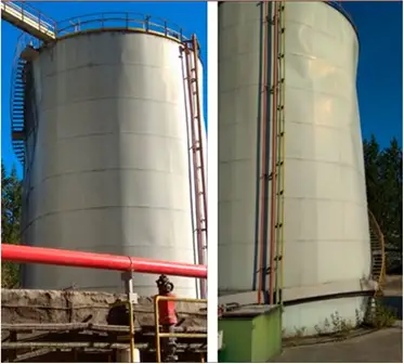
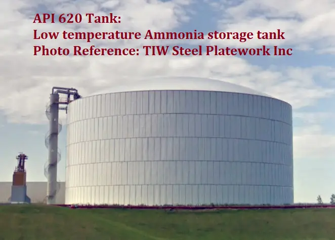
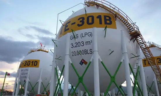
In refineries, petrochemical plants, power plants, process terminals and many other places where the chances of fire are high, various codes and standards (like NFPA) suggest the licensor use fireproofing. For that purpose, Equipment and structures are fireproofed up to a certain height or whole equipment as dictated by guidelines. Refer to Fig. 1, which shows the whole equipment is fireproofed.
Reason for Fireproofing – Why do we do fireproofing?
There are various reasons to do fireproofing equipment and structures. Some of those are listed below:
- To full filling, the industrial requirement of completing NFPA (National fire protection academy) & OSHA requirement
- To increase the resistance of fire
- To keep equipment and critical control systems operating during the Fire.
It is believed that at around 1000°F (538°C), the structural steel loses roughly 50% of its design strength. So by using fireproofing the time to reach that temperature is prolonged. Just to note that a normal fire normally burns in the 1800°F to 2000°F range.
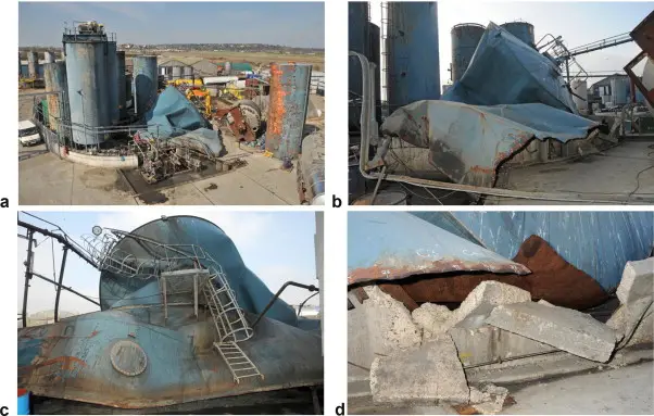
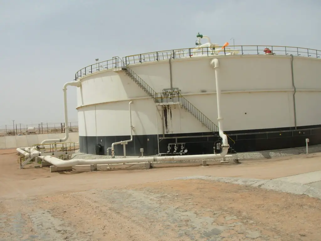
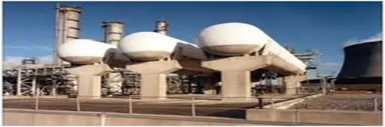
Refer to Fig. 2 which shows the fireproofing in equipment after a certain height.
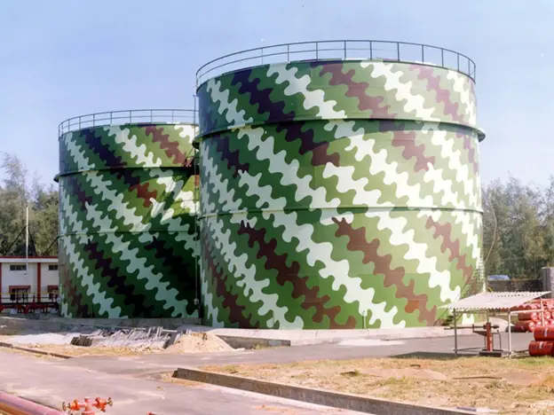
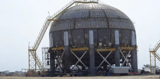
Similarly, in Fig. 3, The fireproofing has been done only in columns and the down portion of spheres as per guidelines.
Fireproofing Codes and Standards
Below mentioned Codes and standards provide guidelines for fireproofing applications:
- BS 476: Part 20-24, Test Methods, and Criteria for the Fire Resistance of Elements of Building Construction.
- API 2218: Fireproofing Practices in Petroleum & Petrochemical Processing Plants
- API 2510: Design and Construction of LPG Installation (Section 10.7)
- NFPA 30: Flammable and Combustible Liquids code
- NFPA 58: Liquefied Petroleum Gas code
- Loss Prevention in the Process Industries by F P Lees, 2nd edition
- International Building Code
- ASTM E119, Fire Tests of Building Construction and Materials
Fireproofing Materials
The design codes and standards do not provide any direct indication of the material to be used for fireproofing. The material must be durable and corrosion-resistant. Based on construction practice, the following materials are used as fireproofing materials:
- Gypsum plasters
- Pyrocrete 241
- Mesh
- Cementitious plasters
- Carbomastic 801(a+b)
- Carboguard 890 (a+b)
- Carboguard 1340 (a+b)
- Carboline 139 (ral 7042)
- Fibrous plasters containing either mineral wool or ceramic fibers
- Thinner # 2
- Thinner # 76
- Thinner #25
- Thinner # 33
- Concrete
- Intumescent coatings
- Asbestos
Fireproofing application method
The following steps are performed for applying fireproofing in mechanical equipment:
- Do the equipment surface preparation
- Apply the primer up to 65 -75 microns.
- Fix nut by tack weld to keep tie mesh.
- Apply Pyrocrete 241
- Apply 2 coats of epoxy paint and check the DFT of the paint as well as the thickness of the fireproof.
- If it is accepted by the engineer in charge or SOP then Vessel can be released for further work.
Types of Fireproofing / Fireproofing types
In many industrial facilities, to secure any insurance fireproofing is a pre-requisite. On a broad scale, Fireproofing is divided into two groups:
- Active Fireproofing and
- Passive Fireproofing
In the case of active fireproofing, human intervention is required for some kind of action to activate the fireproofing system. Whereas, passive fireproofing is planned and designed considering safety plans beforehand. The most common type of passive fireproofing is
- cementitious fireproofing,
- intumescent fireproofing and
- firestop fireproofing.
Cementitious Fireproofing:
These are gypsum-based, plaster-like coatings that look like white stucco when dried. These coatings are sprayed on the structural surfaces requiring fireproofing. Cementite fireproofing is used to keep structural girders and beams below 540 C, where the steel will bend.
Intumescent Fireproofing:
When heated, intumescent paints expand and form a heat-resistant barrier. They usually contain sodium silicates. Under high heat conditions, the intumescent paint coating thickens, entraining air and forming a layer of greater insulation. Intumescent fireproofing paints are used on metallic pipes, tanks, and valves.
Firestop Fireproofing:
In Firestop fireproofing, all openings and joints are sealed with fire-resistance-rated walls and floors. Fire dampers are used to fill the ductwork holes, Hole cuts for pipes, and electrical wiring trays.
Comparison of Cementitious and Intumescent Fireproofing
Intumescent fireproofing is easier to apply than cementitious fireproofing. As they are applied similarly to traditional coating, moisture can not settle inside. As Cementitious fireproofing is done using inexpensive materials, they are applied for fireproofing facilities under some circumstances. However, from a technical standpoint, intumescent fireproofing is more advanced and offers the flexibility of added fire protection.
Required resources for fireproofing
While fireproofing mechanical equipment following resources are required:
- Air compressor- 2 nos
- Hopper- 2 nos
- Spray machine-4 nos
- Compressor for fireproofing- 4 nos
- Mixer machine-3 nos
Even after a simple fireproofing application, it may not work properly due to the following reasons
- Failure of the compressor –Always use TPI inspected Machine for applying Pyrocrete & Paint Properly.
- Over/less application- over-applying Pyrocrete or Painting would cause mud cracking & less application may cause peel-off or orange peel.
- Lack of expertise- Lack of SME (Subject matter expert) may cause repair or failure.
- Lack of Curing- To achieve the milestone or Target sometimes people overtake curing time which may cause repair or Fail.